What Are People Sayin' About Instagram Lite?

In the beginning of May, I used RSelenium to scrape the Google Play Store reviews for Instagram Lite to demonstrate how the package can be used to automate browser behavior. Its taken longer than I had initially planned to do this follow-up on the analysis of that data. But better late than never. So in this analysis I will do some exploratory work and some text mining to look at questions such as:
- How have IG Lite reviews been trending?
- What are prevalent topics in the Google Play reviews about IGLite?
- For words with negative sentiment, why are people feeling negatively?
- What are the most prevalent keywords in the set of reviews?
The main libraries that I will use to do this analysis are udpipe for applying the language model used to develop part of speech tagging, BTM to construct the Biterm model, and textrank / wordcloud to do keyword extraction and make the wordcloud. Both udpipe, BTM, and textrank are part of the Bnosac NLP ecosystem.
The analyses from these posts are heavily inspired from Bnosac’s posts on Biterm Modeling and Sentiment Analysis.
library(tidyverse)  # General Data Manipulation
library(lubridate) # Date Manipulations
library(extrafont)  # To use more fun fonts in GGPLOT
loadfonts(device = "win")
library(udpipe) # Tokenizing, Lemmatising, Tagging and Dependency Parsing
library(BTM) # Biterm Topic Modeling
library(scales) # To help format  plots
library(textrank) # Keyword Extraction
library(wordcloud) # Create wordcloud
For data I’ll be using the result file from the my web scraping post from April:
iglite <- read_csv('https://raw.githubusercontent.com/jtlawren67/jlawblog/master/content/post/2021-05-03-scraping-google-play-reviews-with-rselenium/data/review_data.csv')As a reminder the data looks like:
| names | stars | dates | clicks | reviews |
|---|---|---|---|---|
| Harikrishnan | 3 | 2021-04-05 | 4787 | Its surely consumes less data than original app, but many of you may not get comfortable with this interface. One of the major problems I faced was that stories are getting replayed many times without me doing anything. The next major issue is that if you dont like a post it comes to your feed everytime over and over again until you like the post. Hope Instgram Team will find a solution to these problems |
| Piyush AryaPrakash | 1 | 2021-04-06 | 3655 | It’s good to see that they are providing a lite version. But it doesn’t even work . It’s better to use in chrome than downloading lite. What’s the problem - The feeds never get refreshed . You just have to scroll down and when you click refresh still you see the same feeds. Doesn’t support links . Lags too much . Too much annoying while using the messenger. Despite having a good internet connection it keeps laging saying something went wrong. It’s too slow |
| Badri narayan | 4 | 2021-04-24 | 40 | Very nice app as it is lite so it is good consume less data have limited things but I don’t understand you can watch reels in app but if someone send you reels it shows not supported in lite so it should be fixed and during dark mode the text we type is not visible fix this too and everything is good <U+0001F917> |
Exploring the IG Lite Review Data
Given the time the initial analysis was run I captured 2,040 reviews covering dates from 2019-03-03 and 2021-04-24. However, reviews from earlier than December 2020 are likely referring to the initial version of IG Lite rather than the relaunched version.
The first thing to look at is to see how the review counts have been trending over time:
iglite %>%
  count(dates, name = "reviews") %>%
  filter(dates >= lubridate::ymd(20201201)) %>%
  ggplot(aes(x = dates, y = reviews)) +
    geom_line() +
    geom_smooth(se = F, lty = 2) +
    labs(y = "# of Reviews in data set", x = "Month",
         title = "Number of IGLite Reviews In Dataset") +
    cowplot::theme_cowplot() +
    theme(
      plot.title.position = 'plot',
      text = element_text(family = 'Arial Narrow')
    )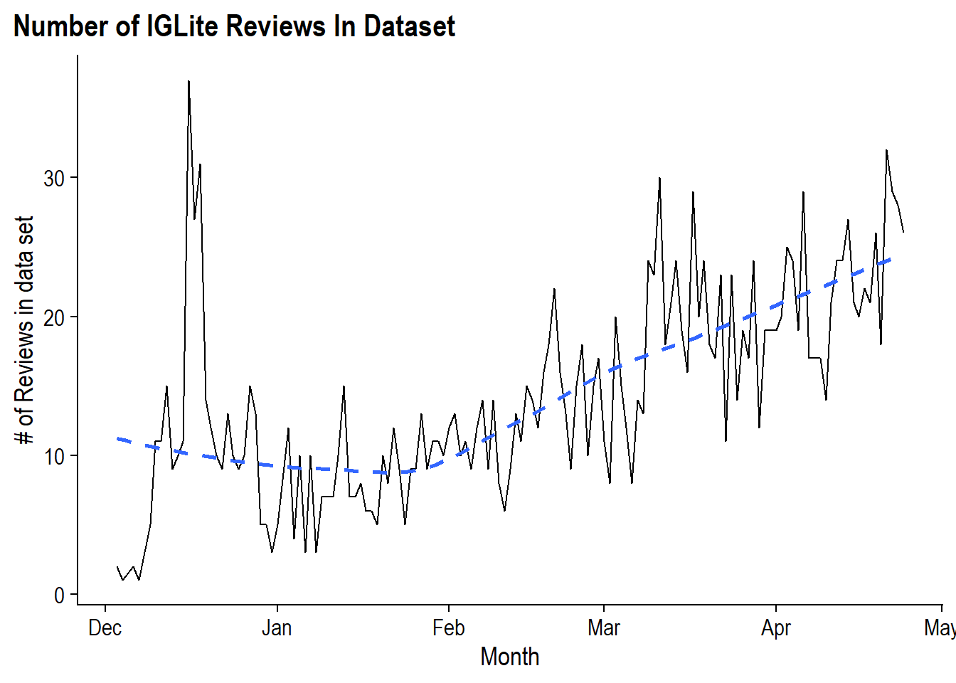
The trend of reviews started strong in mid-December upon the launch of IG Lite before stabilizing at around 10 per day before beginning an incline in February and reaching around 20 reviews per day. So if we assume that increasing reviews are correlated with increasing users then it seems like IG Lite is gaining momentum.
But are the reviews good reviews? As an app that is continuously iterating it would be interesting to see how the distribution of Star Ratings from 1-5 to changed over time as more reviews come in. To do this we can look at the cumulative distributions for each star rating from Dec 2020 through April 2021.
Since certain days do not have coverage across all 5 reviews (remember we’ll only getting 10 per day at the beginning). I’ll need to create a skeleton for each day and all five ratings so that zeros are taken into account rather than treated as gaps. For this I’ll using tidyr’s crossing() function, which is a bit like expand.grid() in Base R to create a data set with all combinations of vectors.
#Create a data frame with every day from 12/1/2020 through the max date and 1-5
#value for stars on each day
tidyr::crossing(
dates = seq.Date(ymd(20201201), max(iglite$dates), by = 'day'),
stars = 1:5
) %>%
# Join actual data to the skeleton to get the number of reviews for that day
left_join(
iglite %>%
count(dates, stars, name = "reviews") %>%
filter(dates >= lubridate::ymd(20201201)),
by = c("dates", "stars")
) %>%
# Fill any missing values with 0
replace_na(list(reviews = 0)) %>%
# Create the cumulative count of reviews for each star level
group_by(stars) %>%
arrange(dates) %>%
mutate(cuml_stars = cumsum(reviews)) %>%
ungroup() %>%
# Add a column for the cumulative count of reviews for up to that point
add_count(dates, wt = cuml_stars, name = "total_review_in_date") %>%
# Create the cumulative distribution for that star level to that point
# For the most recent day create a label to be used in the post
mutate(pct = cuml_stars / total_review_in_date,
lbl = if_else(dates == max(dates),
paste(stars, pct %>% percent(accuracy = 1), sep = ': '),
NA_character_)) %>%
# Remove the dates prior to having 25 total reviews
filter(total_review_in_date >= 25) %>%
# Plot the distribution
ggplot(aes(x = dates, y = pct, color = as.factor(stars))) +
geom_line() +
ggrepel::geom_label_repel(aes(label = lbl)) +
scale_color_discrete(guide = F) +
scale_y_continuous(labels = percent) +
labs(title = "IGLite Rating Distribution",
subtitle = "Cumulative Distribution Dec - Apr",
caption = "Dates Start at 25 Reviews") +
cowplot::theme_cowplot() +
theme(
plot.title.position = 'plot',
text = element_text(family = 'Arial Narrow')
)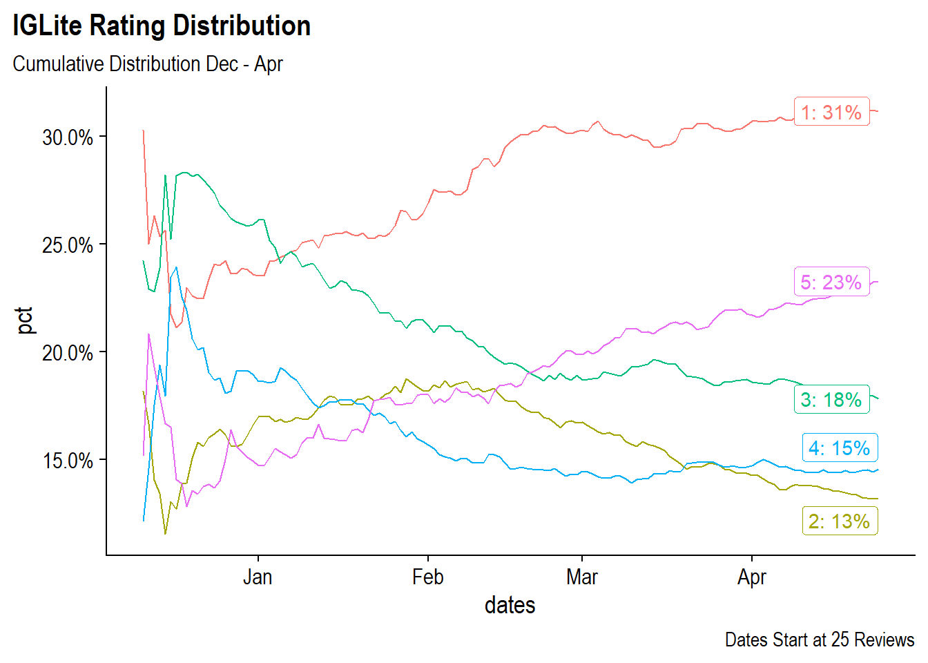 Looking at the distributions over time, in January one and three star ratings were the most common with around 25% each. Fives and twos were relatively low. However, since January, the number of fives have climbed to eventually make up 23% of the total reviews in the data set. Unfortunately, the number of one star reviews has also climbed and is the most common review in the data set at 31%.
An alternative way of utilizing the star ratings is to create a Net Promoter-like score. If you’ve ever received an email asking “On a scale from 1 to 10 how likely are you to recommend this to a friend”, you’ve been a part of the Net Promoter Score. The Net Promoter Score is a score from -100 to 100 that is an index about how willing people are to reccomend a product. It divides the world into Promoters (scores 9 and 10) and Detractors (scores 6 and below) and then calculates % of Promoters - % of Detractors.
In this case, I’ll consider a promoter as someone who rates IGLite a 4 or a 5 and a detractor someone who rates IGLite a 1 or a 2. Then we can calculate our version of NPS for each month to get a rough look at sentiment trend.
iglite %>%
  # Filter to December
  filter(dates >= lubridate::ymd(20201201)) %>%
  # Turn star scores into Promoter / Detractors and create a dataset where
  # for each day we'll have Favorable/Unfavorable/Neutral as columns
  mutate(lbl = case_when(
    stars >= 4 ~ "favorable",
    stars <= 2 ~ "unfavorable",
    TRUE ~ "neutral"
    ),
    mth = format(dates, "%Y-%m")
  ) %>%
  count(mth, lbl, name = "reviews") %>%
  spread(lbl, reviews) %>%
  replace_na(list(favorable = 0, unfavorable = 0, neutral = 0)) %>%
  # Calculate the NPS score
  mutate(
         total = favorable + neutral + unfavorable,
         pct_favorable = favorable/total,
         pct_unfavorable = unfavorable/total,
         nps = pct_favorable - pct_unfavorable
         ) %>%
  # Plot the NPS score by month
  ggplot(aes(x = mth, y = nps), group = 1) +
    geom_col(aes(fill = if_else(nps < 0, 'darkred', 'darkgreen'))) +
    geom_point() +
    geom_label(aes(label = nps %>% percent(accuracy = .1))) +
    scale_fill_discrete(guide = F) +
    labs(title = "NPS Score for IGLite",
         subtitle = "NPS = % Promoters (Reviews > 3) - % Detractors (Reviews < 3)",
         y = "Net Promoter Score",
         x = "Month") +
   cowplot::theme_cowplot() +
    theme(
      plot.title.position = 'plot',
      text = element_text(family = 'Arial Narrow'),
      axis.text.y = element_blank(),
      axis.ticks.y = element_blank()
    )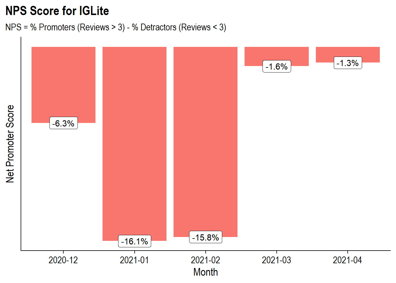
Yikes! This does not look great with each of the 5 months in the data having a negative NPS score. However, similar to the cumulative ratings in the chart above the later months (March and April) have faired much better than the first two months post-release (Jan and Feb) with the NPS score being close to zero. Looking at the raw data, it seems like the “neutral” comes from being polarizing with 42% Promoters and 43% Detractors rather than having a lot of people with neutral with 3 star ratings:
| Month | Total Reviews | % Favorable | % Neutral | % Unfavorable | NPS |
|---|---|---|---|---|---|
| 2020-12 | 301 | 33.9% | 25.9% | 40.2% | -6.3% |
| 2021-01 | 248 | 33.9% | 16.1% | 50.0% | -16.1% |
| 2021-02 | 361 | 34.6% | 15.0% | 50.4% | -15.8% |
| 2021-03 | 565 | 40.0% | 18.4% | 41.6% | -1.6% |
| 2021-04 | 540 | 41.7% | 15.4% | 43.0% | -1.3% |
Text-Mining
With the EDA portion done, its on to Text Mining the reviews. In a past-post I had used the Tidytext Ecosystem to look at Tweet difference between Instagram and TikTok but this time I will be using the Bnosac ecosystem of packages to do Biterm Modeling, Sentiment Analysis with dependency parsing, and then the textrank and wordcloud package to generate a word-cloud of extracted keywords.
Pre-processing with udpipe
In prior text-mining posts, I used tidytext to handle tokenization, however, in this analysis I will leverage the udpipe package. The udpipe is a R wrapper around the C++ library of the same name that uses a pre-trained language models to easily tokenize, tag, lemmatize or perform dependency parsing on text in any language. The “ud” in udpipe stands for Universal Dependencies which is a “framework for consistent annotation of grammar”.
In order to prepare the data for the model there needs to be some light pre-processing as udpipe expects the data to have a doc_id and a text field.
#Columns need to be doc_id and text for the model
cleaned <- iglite %>%
  mutate(doc_id = row_number(),
         text = str_to_lower(reviews),
         text = str_replace_all(text, "'", ""))
To annotate our data with udpipe I’ll call the udpipe() function with my data and the language of the model to use. This function is will download the appropriate language model, in this case English, and then annotate the data.
annotated_reviews <- udpipe(cleaned, "english")To show what the udpipe model did to the data we can look at the first review before the annotations:
| text |
|---|
| its surely consumes less data than original app, but many of you may not get comfortable with this interface. one of the major problems i faced was that stories are getting replayed many times without me doing anything. the next major issue is that if you dont like a post it comes to your feed everytime over and over again until you like the post. hope instgram team will find a solution to these problems |
and after the annotations:
annotated_reviews %>% filter(doc_id == 1) %>% head(3) %>% knitr::kable()| doc_id | paragraph_id | sentence_id | sentence | start | end | term_id | token_id | token | lemma | upos | xpos | feats | head_token_id | dep_rel | deps | misc |
|---|---|---|---|---|---|---|---|---|---|---|---|---|---|---|---|---|
| 1 | 1 | 1 | its surely consumes less data than original app, but many of you may not get comfortable with this interface. | 1 | 3 | 1 | 1 | its | its | PRON | PRP$ | Gender=Neut|Number=Sing|Person=3|Poss=Yes|PronType=Prs | 3 | nsubj | NA | NA |
| 1 | 1 | 1 | its surely consumes less data than original app, but many of you may not get comfortable with this interface. | 5 | 10 | 2 | 2 | surely | surely | ADV | RB | NA | 3 | advmod | NA | NA |
| 1 | 1 | 1 | its surely consumes less data than original app, but many of you may not get comfortable with this interface. | 12 | 19 | 3 | 3 | consumes | consume | VERB | VBZ | Mood=Ind|Number=Sing|Person=3|Tense=Pres|VerbForm=Fin | 0 | root | NA | NA |
We now get a ton of metadata including indicators for the sentence, we can the token (token) and its lemma (lemma) (note that consumes becomes consume), parts of speech (upos), and dependency relationships (deprel) and more.
Now that we’ve tokenized the data we can start using it to analyze the reviews.
Biterm Modeling
The first analysis task will be biterm modeling using the BTM package. The Biterm Topic Model model was developed by Yan et. al as a means to determining the topics that occur in short-texts such as Tweets (or in this case Google Play Reviews). Its meant to provide an improvement to traditional topics modeling in uses cases such as this. My understanding of the difference between traditional topic modeling and biterm topic model is that in the former, the model learns word co-occurrence within documents, while with the later, the model learns word co-occurrences within a window across the entire set of documents. In this context a “biterm” consists of two words co-occurring in the same context, for example, in the same short text window. This analysis is modeled after the one from bnosac.
In the BTM model we can explicitly tell the model which word co-occurrences we care about vs. letting it run on everything. This enables us to only care about certain parts of speech, words of certain lengths, and non-stop words. For this analysis we will consider a co-occurrence window of 3 while removing stopwords, removing words with less than 3 characters, and only keeping nouns, adjectives, verbs, and adverbs.
#Define a Dictionary of BiTerms
library(data.table)
library(stopwords)
biterms <- as.data.table(annotated_reviews)
biterms <- biterms[, cooccurrence(x = lemma,
                                  relevant = upos %in% c("NOUN", "ADJ", "VERB") &
                                             nchar(lemma) > 2 & !lemma %in% stopwords("en"),
                                  skipgram = 3),
                   by = list(doc_id)]
The biterm data set we’ve constructed looks like:
biterms %>% head(5) %>% knitr::kable()| doc_id | term1 | term2 | cooc |
|---|---|---|---|
| 1 | like | post | 2 |
| 1 | consume | less | 1 |
| 1 | less | data | 1 |
| 1 | original | app | 1 |
| 1 | get | comfortable | 1 |
This states that in the first review, the word pair (like, post) occurs within a 3 word window twice in the document.
Now we can actually construct the biterm model. For simplicity, I’m setting it to train 9 topics. The background = T setting makes the 1st topic a background topic that reflects to empirical word distribution to filter out common words (which is why k = 10):
set.seed(123456)

train_data <- annotated_reviews %>%
  filter(
    upos %in% c("NOUN", "ADJ", "VERB"),
    !lemma %in% stopwords::stopwords("en"),
     nchar(lemma) > 2
  ) %>%
  select(doc_id, lemma)

btm_model     <- BTM(train_data, biterms = biterms, k = 10, iter = 2000, background = TRUE)
Now that we’ve constructed topics, there needs to be a good way to visualize those topics. Fortunately the textplot package handles this nicely:
library(textplot)
library(ggraph)
set.seed(123456)
plot(btm_model, top_n = 10,
title = "BTM model of IGLite Reviews",
labels = c("",
"Reels",
"Likes the App",
"Takes Too Long",
"Can't Upload",
"Dark Mode",
"Bugs",
"Feature Requests",
"Uses Less Resources",
"Instagram Lite"))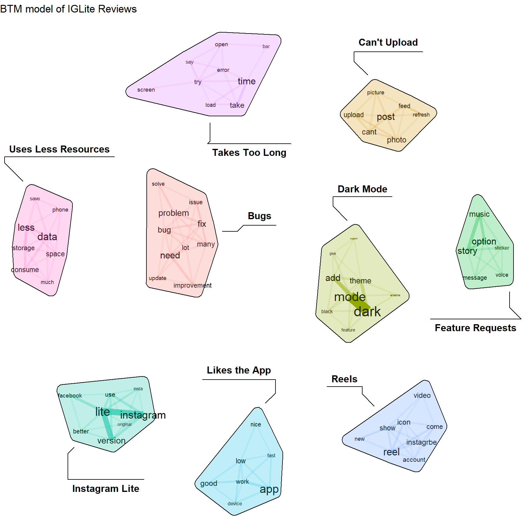 From this chart we can see that there’s a lot of people mentioning bugs and other problems, specifically around upload. People talking about how IG Lite consumes less space and data, people wanting new features such as a music sticker option in stories, and a LOT of people wanting Dark Mode. And there are people who like it and think its a good app.
Sentiment Analysis withe Dependency Parsing
In many sentiment analyses a dictionary method is used to assign positive sentiment and negative sentiment and then some sort of aggregation occurs to determine whether a document is “happy” or “sad” or whatever other type of emotion. But what gets left on the table is “Why” there is positive or negative sentiment. In this case, we can see that people gave IG Lite bad ratings or complained about issues, but without looking through every review, it tough to know why.
This next piece is based on a bnosac blog post and will leverage the dependency output from udpipe to see what words are connected to the words with negative sentiment.
To first determine words with negative sentiment I will need an external dictionaries to identify:
- Positive vs. Negative words - the base positive vs. negative scoring
- Amplifying and Deamplifying words - words like ‘very’ which make an emotion more intense or ‘barely’ which make an emotion less intense.
- Negators - words like ‘not’ which would flip the sentiment
For these lists I will get the data used in the sentometrics package:
load(url("https://github.com/SentometricsResearch/sentometrics/blob/master/data-raw/FEEL_eng_tr.rda?raw=true"))
load(url("https://github.com/SentometricsResearch/sentometrics/blob/master/data-raw/valence-raw/valShifters.rda?raw=true"))
and break them up into separate vectors of words:
polarity_terms <- FEEL_eng_tr %>% transmute(term = x, polarity = y)
polarity_negators <- valShifters$valence_en %>% filter(t==1) %>% pull(x) %>% str_replace_all("'","")
polarity_amplifiers <- valShifters$valence_en %>% filter(t==2) %>% pull(x) %>% str_replace_all("'","")
polarity_deamplifiers <- valShifters$valence_en %>% filter(t==3) %>% pull(x) %>% str_replace_all("'","")
Finally, I can use udpipe’s txt_sentiment function to use these lists to score my annotated data.
sentiments <- txt_sentiment(annotated_reviews, term = "lemma",
                            polarity_terms = polarity_terms,
                            polarity_negators = polarity_negators,
                            polarity_amplifiers = polarity_amplifiers,
                            polarity_deamplifiers = polarity_deamplifiers)
sentiments <- sentiments$data
In addition to the initial annotations there are now columns for polarity (just the positive / negative based on the term) and sentiment_polarity which incorporates the additional information.
Now that there are sentiments I’m going to want to find the words that those negative terms modify using cbind_dependencies().
reasons <- sentiments %>%
  #Attached Parent Words to Data
  cbind_dependencies() %>%
  #Filter Columns
  select(doc_id, lemma, token, upos, polarity, sentiment_polarity, token_parent, lemma_parent, upos_parent, dep_rel) %>%
  #Keep Only Terms with Negative Sentiment
  filter(sentiment_polarity < 0)
The revised data now looks like:
head(reasons) %>% knitr::kable()| doc_id | lemma | token | upos | polarity | sentiment_polarity | token_parent | lemma_parent | upos_parent | dep_rel |
|---|---|---|---|---|---|---|---|---|---|
| 1 | less | less | ADJ | -1 | -1.8 | data | data | NOUN | amod |
| 1 | comfortable | comfortable | ADJ | 1 | -1.0 | get | get | VERB | xcomp |
| 1 | problem | problems | NOUN | -1 | -1.0 | one | one | NUM | nmod |
| 1 | do | do | AUX | 1 | -1.0 | like | like | VERB | aux |
| 1 | problem | problems | NOUN | -1 | -1.0 | solution | solution | NOUN | nmod |
| 2 | do | does | AUX | 1 | -1.0 | work | work | VERB | aux |
A quick look at the data calls out a problem that exists with all dictionary based approaches which is that there is a context that the analyst knows that a dictionary cannot. For example, the term above “less data” is taken to be a negative because having “less data” would be bad… except in the context of Instagram Lite using “less data” would actually be good.
To get a better understanding of why we’re seeing negative sentiment I will construct a network graph between the negative term and the thing they are modifying and looking for the common phrases.
# Keep only dependency relationships that are adjectival modifiers
# (terms that modify a noun / pronoun)
reasons <- filter(reasons, dep_rel %in% "amod")
# Count Number of occurrences
word_cooccurences <- reasons %>%
count(lemma, lemma_parent, name = "cooc", sort = T)
# Create the Nodes as either the term in the dictionary or a word linked
#to the term in the dictionary
vertices <- bind_rows(
data_frame(key = unique(reasons$lemma)) %>%
mutate(in_dictionary = if_else(key %in% polarity_terms$term,
"in_dictionary",
"linked-to")),
data_frame(key = unique(setdiff(reasons$lemma_parent, reasons$lemma))) %>%
mutate(in_dictionary = "linked-to")
)
library(ggraph)
library(igraph)
# Keep Top 20 Words CoOccurances
cooc <- head(word_cooccurences, 20)
set.seed(123456789)
cooc %>%
graph_from_data_frame(vertices = filter(vertices,
key %in% c(cooc$lemma,
cooc$lemma_parent))) %>%
ggraph(layout = "fr") +
geom_edge_link0(aes(edge_alpha = cooc, edge_width = cooc)) +
geom_node_point(aes(color = in_dictionary), size = 5) +
geom_node_text(aes(label = name), vjust = 1.8, col = "darkgreen") +
scale_color_viridis_d(option = "C", begin = .2, end = .8) +
ggtitle("Which words are linked to the negative terms") +
theme_void()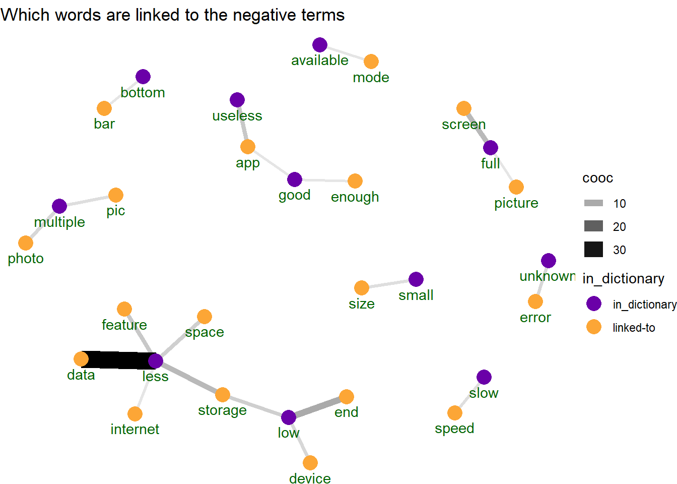 In the network we see the “less data” as the strongest co-occurrence even thought it (and many other words in this group) are not strictly negative words. Some of these connections make sense to be negative like “slow speed” or “useless app” which seems unquestionably bad. But some of these don’t make sense to me like “full screen” being bad. Although looking at a few of the sample reviews that say full screen they are usually in reference to full screen modes not working. So while it does appear that the sentiment model is capturing that “full screen” is discussed as a negative thing, the graph view above does not make that clear.
So dependency parsing for sentiment analysis seems like a cool idea but is a bit “your mileage may vary”.
Word Clouds on Keywords
The last text analysis technique for this post will probably be the most well known… wordclouds. It will show what are the most common words in our data set and can be used to understand the set of reviews at a quick glance. But rather than relying on most common words, I’ll use the textrank package to extract relevant keywords text where keywords are defined as combinations of words following each other. To try to get the most relevant set of keywords, I will be limiting to nouns, adjective, and verbs and will create a wordcloud of the top 30.
textrank_keywords(annotated_reviews$lemma,
                  relevant = annotated_reviews$upos %in% c('NOUN', 'ADJ', 'VERB')) %>%
  .$keywords %>% filter(ngram > 1 & freq > 1, !str_detect(keyword, 'be')) %>%
  slice_max(freq, n = 50) %>%
  with(wordcloud(keyword, freq, max.words = 50, colors = brewer.pal(10, 'Dark2')))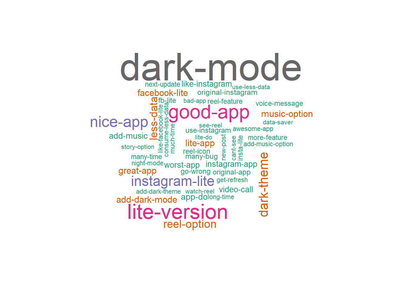
So what are people saying about IG Lite…. that they want dark mode, they want music stickers and that its a good app.
Conclusions
In this post I leveraged the Google Play Reviews that were scraped back in April to analyze the ratings and the review text using some of less well-known NLP packages (at least in my opinion) to do modified versions of Topic Modeling with Biterm Models, modified versions of sentiment analysis with dependency parsing, and a modified version of a word cloud using keyword extraction.
As far as answering the questions about what are people saying about IG Lite. It seems really mixed. In terms of star ratings things appeared to start very rough in Jan / Feb but had improved through March and April. From the topic models, some people like that its less resource intense than “Instagram Heavy” while others find it buggy and lacking features. From the sentiment analysis, this polarized view can be summed up in the nodes that formed “Good App”, “Good Enough”, and “Useless App” such that there’s no dominant sentiment.
Except Dark Mode… give the people dark mode.