What's the Difference Between Instagram and TikTok? Using Word Embeddings to Find Out

TL;DR
- Instagram - Tiktok = Photos, Photographers and Selfies
- Tiktok - Instagram = Witchcraft and Teens
but read the whole post to find out why!
Purpose
The original intent of this post was to learn to train my own Word2Vec model, however, as is a running theme.. my laptop is not great and training a neural network would never work. However, in looking for alternatives, I had come across a post from Julia Silge from 2017 which outlined how create Word Embeddings using a combination of point-wise mutual information (PMI) and Singular Value Decomposition (SVD). This was based on a methodology from Chris Moody’s Stitchfix Post called Stop Using word2vec. Ms. Silge’s methodology has been updated as part of her book Supervised Machine Learning for Text Analysis in R.
Word Embeddings are vector representations of words in a large number of dimensions that capture the context of how words are used. They have been used to show fancy examples of how you can do math with words. One of the most well known example is King - Man + Woman = Queen.
Since TikTok and Instagram are both popular social media apps, especially among teenagers, I figured it would be an interesting exercise to see if I could figure out Tiktok - Instagram = ???? and Instagram - TikTok = ????.
Getting and Cleaning the Data
In order to create these vector representations I need data. In the example posts above, they use the Hacker News corpus which is available on Google’s BigQuery. In quickly browsing that data it didn’t seem like there was enough to do something as targeted as Instagram vs. TikTok. So I decided to use Twitter data both because I thought it would be a decent source of information and second because it was a good excuse to try out the rtweet package.
In addition to the rtweet package, I’ll be using tidyverse for data manipulations and plotting, tidytext to create the word tokens, and widyr in order to do the PMI, SVD, and Cosine Similarity calculations.
library(rtweet) # To Exract Data from Twitter
library(tidyverse) # Data Manipulation and Plotting
library(tidytext) # To create the Work Tokens and Bigrams
library(widyr) #For doing PMI, SVD, and Similarity
Turns out getting data from Twitter really couldn’t be easier with rtweet. The search_tweets() function is very straight forward and really is all you need. In this case, I wanted to run two separate queries, one for “instagram” and one for “tiktok”, so I used search_tweets2() which allows you to pass a vector of queries rather than a single one. In the code below, my two queries, one for “instagram” and one for “tiktok” are captured in the q parameter (with additionally filters to remove tweets with links and tweets with replies). The n parameter says that I want 50,000 tweets for each query. Additionally, I tell the query that I don’t want retweets, I want to grab recent tweets (the package can only search the last 6-7 days), and I want only English language.
tweets <- search_tweets2(
  q = c("tiktok -filter:quote -filter:replies -filter:links",
        'instagram -filter:quote -filter:replies -filter:links'),
  n = 50000,
  include_rts = FALSE,
  retryonratelimit = TRUE,
  type = 'recent',
  lang = 'en'
)
The query for this data was originally run on 7/21/2020 and returned 108,000 rows. Because the Twitter data contains many characters not typically considered words, the data was run through some data cleaning and duplicated tweets (ones that contained both “instagram” and “tiktok” were deduped.
cleaned_tweets <- tweets %>%
#Encode to Native
transmute(status_id, text = plain_tweets(text)) %>%
#Remove Potential Dups
distinct() %>%
#Clean Data
mutate(
text = str_remove_all(text, "^[[:space:]]*"), # Remove leading whitespaces
text = str_remove_all(text, "[[:space:]]*$"), # Remove trailing whitespaces
text = str_replace_all(text, " +"," "), # Remove extra whitespaces
text = str_replace_all(text, "'", "%%"), # Replacing apostrophes with %%
#text = iconv(text, "latin1", "ASCII", sub=""), # Remove emojis/dodgy unicode
text = str_remove_all(text, "<(.*)>"), # Remove pesky Unicodes like <U+A>
text = str_replace_all(text, "\\ \\. ", " "), # Replace orphaned fullstops with space
text = str_replace_all(text, " ", " "), # Replace double space with single space
text = str_replace_all(text, "%%", "\'"), # Changing %% back to apostrophes
text = str_remove_all(text, "https(.*)*$"), # remove tweet URL
text = str_replace_all(text, "\\n", " "), # replace line breaks with space
text = str_replace_all(text, "&", "&"), # fix ampersand &,
text = str_remove_all(text, '<|>'),
text = str_remove_all(text, '\\b\\d+\\b') #Remove Numbers
) Finally, the data was tokenized to break apart the tweets into a tidy format of 1 row per word. For example, “The quick brown fox” will be broken into 4 rows, the first containing “the”, the second containing “quick” and so on. Besides tokenization, stop words and infrequent words (<20 occurrences) were removed. Stop words are very common words like “the”, “it”, etc. that don’t add much meaning to the Tweets.
tokens <- cleaned_tweets %>%
  #Tokenize
  unnest_tokens(word, text) %>%
  #Remove Stop Words
  anti_join(stop_words, by = "word") %>%
  #Remove All Words Occurring Less Than 20 Times
  add_count(word) %>%
  filter(n >= 20) %>%
  select(-n)
Creating the Embeddings
The way that word embeddings are able to capture the context of individual words is by looking at what words appear around the word of interest. Getting from Tokens to Embeddings are done in three steps:
- Create the Sliding Window to capture words occurring together
- Calculate the point-wise mutual information to provide a measure to how likely two words will appear together
- Use SVD to decompose the matrix of 4,586 words into some number of dimensions (in this case we’ll use 100).
Creating the Sliding Windows
Sliding windows in text is kind of like a rolling average for numbers where at any point there is a subset of data that we’re looking at as subset moves over the entire data set.
A very simple example would be the string “the quick brown fox jumps over the lazy dog” with a window size of four will generate six windows
| window_id | words |
|---|---|
| 1_1 | the, quick, brown, fox |
| 1_2 | quick, brown, fox, jumps |
| 1_3 | brown, fox, jumps, over |
| 1_4 | fox, jumps, over, the |
| 1_5 | jumps, over, the, lazy |
| 1_6 | over, the, lazy, dog |
The examples from the blog post use a combination of nesting and the furrr package to create sliding windows in parallel. Since my laptop only has two cores, there isn’t much benefit to parallelizing this code. Fortunately, someone in the comments linked to this gist from Jason Punyon which works very quickly for me.
slide_windows <- function(tbl, doc_var, window_size) {
  tbl %>%
    group_by({{doc_var}}) %>%
    mutate(WordId = row_number() - 1,
           RowCount = n()) %>%
    ungroup() %>%
    crossing(InWindowIndex = 0:(window_size-1)) %>%
    filter((WordId - InWindowIndex) >= 0, # starting position of a window must be after the beginning of the document
           (WordId - InWindowIndex + window_size - 1) < RowCount # ending position of a window must be before the end of the document
    ) %>%
    mutate(window_id = WordId - InWindowIndex + 1)
}
The one parameter that we need to choose when creating the windows is the window size. There is no right or wrong answer for a window size since it will depend on the question being asked. From Julia Silge’s post, “A smaller window size, like three or four, focuses on how the word is used and learns what other words are functionally similar. A larger window size, like ten, captures more information about the domain or topic of each word, not constrained by how functionally similar the words are (Levy and Goldberg 2014). A smaller window size is also faster to compute”. For this example, I’m choosing a size of eight.
Point-wise Mutual Information
Point-wise mutual information is an association measurement to determine how likely two words are to occur together normalized by how likely each of the words are to be found on their own. The higher the PMI the more likely words are to be found close together vs. on their own.
PMI(word1, word2) = log(P(word1, word2)/(P(word1)P(word2)))
This can be calculated using the pairwise_pmi() function from the widyr package.
Singular Value Decomposition
This final step will turn our set of Word/Word PMI values into a 100-dimensional embedding for each word using Singular Value Decomposition, which is a technique for dimensionality reduction.
This is calculated using the widely_svd() function also from widyr.
Putting it all together
Executing these three steps can done in the following code:
tidy_word_vectors <- tokens %>%
  slide_windows(status_id, 8) %>% #Create Sliding Window of 8 Words (Step 1)
  unite(window_id, status_id, window_id) %>% #Create new ID for each window
  pairwise_pmi(word, window_id) %>%  #Calculate the PMI (Step 2)
  widely_svd(item1, item2, pmi, nv = 100, maxit = 1000) #Create 100 Dimension Embedding (Step 3)
The data at this point looks like:
## # A tibble: 6 x 3
##   item1     dimension    value
##   <chr>         <int>    <dbl>
## 1 instagram         1  0.0273
## 2 instagram         2 -0.0101
## 3 instagram         3 -0.0729
## 4 instagram         4  0.107
## 5 instagram         5 -0.00237
## 6 instagram         6 -0.0844
Where item1 represents the word, dimension is each of our 100 dimensions for the word vector, and value is the numeric value for that dimension for that word.
The Fun Stuff
Now that we have these embeddings, which again are 100-dimensional vectors to represent each word we can start doing analysis to hopefully find some find things.
What Word is Most Similar to Instagram?
To find the most similar words, we can use cosine similarity to determine which vectors are most similar to our target words. Cosine similarity can be calculated using the pairwise_similarity() function from the widyr package.
Let’s look at what’s most similar to “Instagram”:
#Get 10 Most Similar Words to Instagram
ig <- tidy_word_vectors %>%
  pairwise_similarity(item1, dimension, value) %>%
  filter(item1 == 'instagram') %>%
  arrange(desc(similarity)) %>%
  head(10)

#Plot most similar words
ig %>%
  ggplot(aes(x = fct_reorder(item2, similarity), y = similarity, fill = item2)) +
    geom_col() +
    scale_fill_discrete(guide = F) +
    labs(x = "", y = "Similarity Score",
         title = "Words Most Similar to <i style='color:#833AB4'>Instagram</i>") +
    coord_flip() +
    hrbrthemes::theme_ipsum_rc(grid="X") +
    theme(
      plot.title.position = "plot",
      plot.title = ggtext::element_markdown()
    )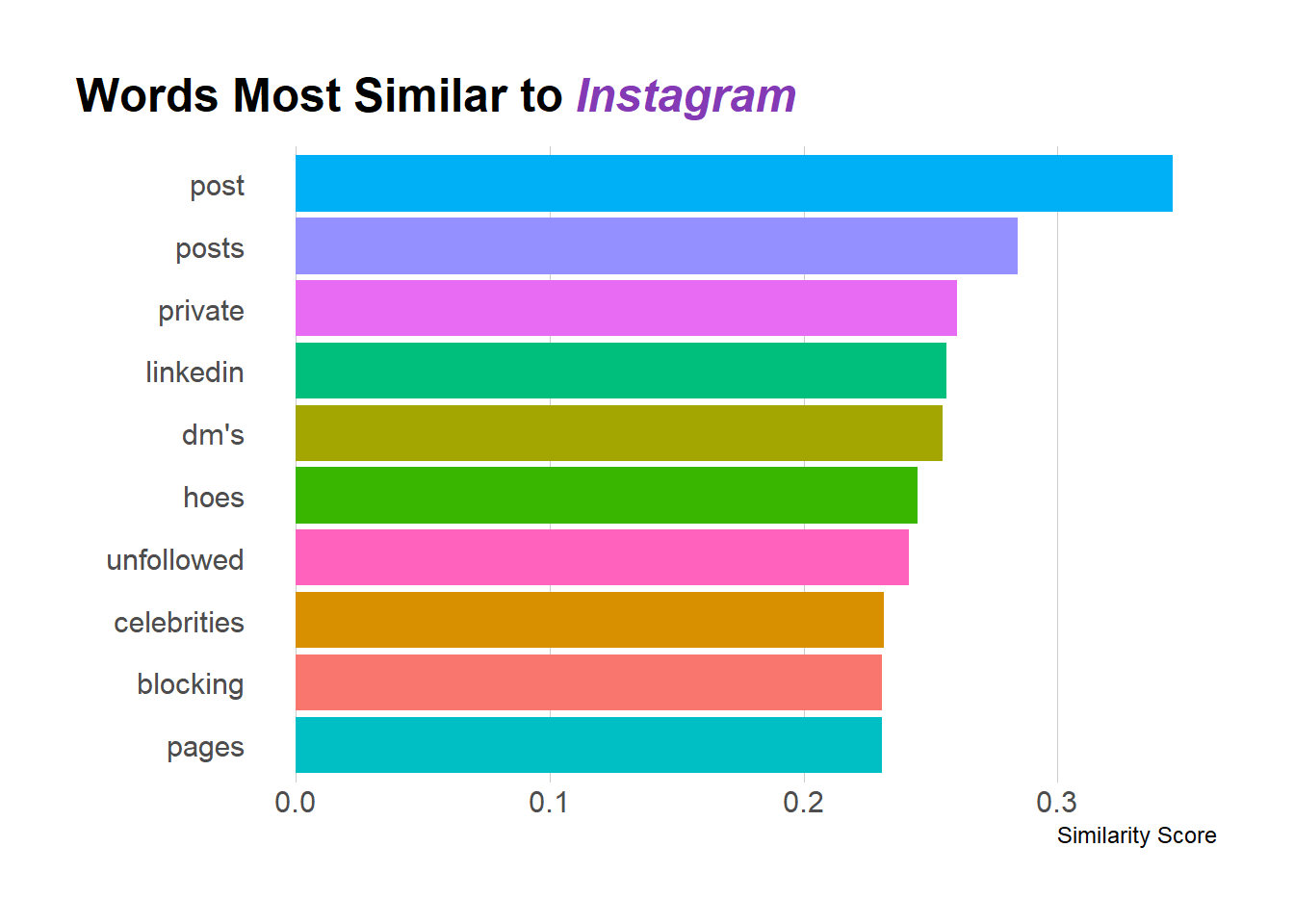
Looking at what words are most similar can provide a good gut check for whether things are working. Among the top words are “post(s)”, “dms”, “celebrities” which all seem to make sense in the context of Instagram. Admittedly, I got a chuckle about “Instagram hoes”, but that does have its own Urban Dictionary definition so I suppose its legit.
What Word is Most Similar to TikTok?
We can do the same calculation with ‘tiktok’ as opposed to ‘instagram’
tt <- tidy_word_vectors %>%
  pairwise_similarity(item1, dimension, value) %>%
  filter(item1 == 'tiktok') %>%
  arrange(desc(similarity)) %>%
  head(10)

tt %>%
  ggplot(aes(x = fct_reorder(item2, similarity), y = similarity, fill = item2)) +
  geom_col() +
  scale_fill_discrete(guide = F) +
  labs(x = "", y = "Similarity Score",
       title = "Words Most Similar to <i style='color:#69C9D0'>TikTok</i>") +
  coord_flip() +
  hrbrthemes::theme_ipsum_rc(grid="X") +
  theme(
    plot.title.position = "plot",
    plot.title = ggtext::element_markdown()
  )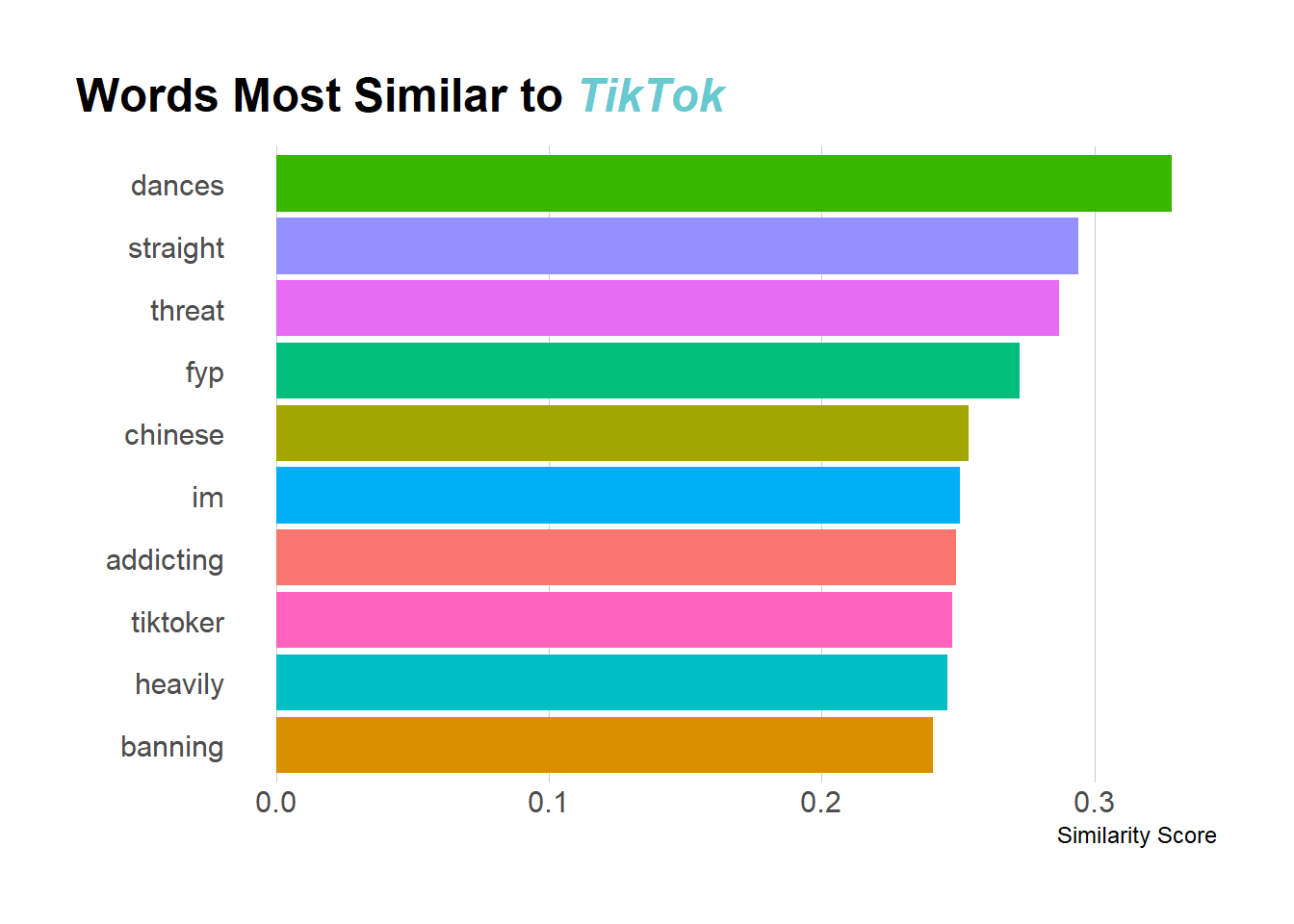
Now admittedly, I’m less familiar with TikTok than I am Instagram, but from what I do know (and what I can Google), these make a lot of sense. The word most similar to TikTok is “dances” and I do know that TikTok is known for its viral dances. Some of the other terms I needed to look up but they seem legit. For example, “Straight TikTok” is used to refer to more mainstream TikTok vs. “Alt Tiktok” and “fyp” is the “For You Page” (I don’t actually know what this is, but I know its something TikTok-y). So again, I feel pretty good about these results.
What is the Difference between TikTok and Instagram?
As mentioned at the start the goal of this post is to create Instagram - Tiktok = ? and Tiktok - Instagram = ? similar to the king - man + woman = queen often referenced in Word2Vec (or other embedding) posts.
Since both TikTok and Instagram are now represented by 100-dimensional numeric vectors doing the subtraction is as simple as doing a pairwise subtraction on each dimension. Since our data is in a tidy format it takes a little bit of data wrangling to pull that off, but ultimately we’re going to grab the Top 10 Closest words to (Instagram-TikTok) and (TikTok-Instagram) by treating these resulting vectors as fake “words” and adding them to the data set before calculating the cosine similarity.
tt_ig_diff <- tidy_word_vectors %>%
  #Calculate TikTok - Instagram
  filter(item1 %in% c('tiktok', 'instagram')) %>%
  pivot_wider(names_from = "item1", values_from = "value") %>%
  transmute(
    item1 = 'tiktok_minus_ig',
    dimension,
    value = tiktok - instagram
  ) %>%
  bind_rows(
    #Calculate Instagram - TikTok
    tidy_word_vectors %>%
    filter(item1 %in% c('tiktok', 'instagram')) %>%
    pivot_wider(names_from = "item1", values_from = "value") %>%
    transmute(
      item1 = 'ig_minus_tiktok',
      dimension,
      value = instagram - tiktok
    )
  ) %>%
  #Add in the rest of the individual words
  bind_rows(tidy_word_vectors) %>%
  #Calculate Cosine Similarity on All Words
  pairwise_similarity(item1, dimension, value) %>%
  #Keep just the simiarities to the two "fake words"
  filter(item1 %in% c('tiktok_minus_ig', 'ig_minus_tiktok')) %>%
  #Grab top 10 most similar values for each "fake word"
  group_by(item1) %>%
  top_n(10, wt = similarity)

#Plotting the Top 10 Words by Similarity
tt_ig_diff %>%
  mutate(item1 = if_else(
    item1 == "ig_minus_tiktok", "Instagram - TikTok = ", "Tiktok - Instagram = "
  )) %>%
  ggplot(aes(x = reorder_within(item2, by = similarity, within = item1),
             y = similarity, fill = item2)) +
  geom_col() +
  scale_fill_discrete(guide = F) +
  scale_x_reordered() +
  labs(x = "", y = "Similarity Score",
       title = "What's the Difference between <i style='color:#833AB4'>Instagram</i>
       and  <i style='color:#69C9D0'>TikTok</i>") +
  facet_wrap(~item1, scales = "free_y") +
  coord_flip() +
  hrbrthemes::theme_ipsum_rc(grid="X") +
  theme(
    plot.title.position = "plot",
    plot.title = ggtext::element_markdown(),
    strip.text = ggtext::element_textbox(
      size = 12,
      color = "white", fill = "#5D729D", box.color = "#4A618C",
      halign = 0.5, linetype = 1, r = unit(5, "pt"), width = unit(1, "npc"),
      padding = margin(2, 0, 1, 0), margin = margin(3, 3, 3, 3)
    )
  )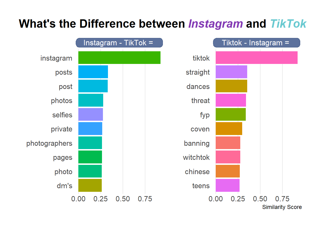
A couple of things jump out from the results. First, the vectors for TikTok and Instagram aren’t similar enough to each other to not make “TikTok” or “Instagram” the most similar value. This is likely because of the data collection methodology of using TikTok and Instagram as search terms on Twitter. Also, as a result of this there is a bit of overlap between the “Most Similar Word to X” and the “Most Similar Word to X-Y”.
However, once you get past the overlaps there are some interesting findings. For Instagram - TikTok you get “Selfies, Photo(s), Photographer” which makes a ton of sense since Instagram is primary a photo app while TikTok is entirely a video app.
For Tiktok - Instagram, there still is a lot of overlap with just TikTok, but for the new items there’s a bunch of Witchcraft terms (coven, witchtok). But according to Wired UK TikTok has become the home of modern witchcraft that seems to track. Also, “Teens” is surfaced as a difference between Tiktok and Instagram reflecting its popularity among US Teenagers.
Concluding Thoughts
I wanted to get involved with Word Embeddings through Word2Vec but I don’t have the technology for it. Luckily resources on the internet provided a way to do this with tools not requiring a Neural Network. By grabbing data from Twitter it was easy to create word embeddings and to try to understand the differences between TikTok and Instagram. In practice it would be good to have had more than 100,000 Tweets and I wish that there was a way to get word context more in the wild than specific search terms. But in the end, I’m happy with the results.