Heatmapping My New York City Marathon Training
Motivation
This post was inspired by my wife who used the GPS data from her Strava app to plot her running routes during 2020. Since I don’t run nearly as much as I used to, I need to go back to when I was training for the NYC marathon to find enough running to make such a map worthwhile. Also presenting a challenge is that I’m a bit of a luddite when it comes to running technology. I don’t have a GPS watch and I don’t run with a phone. To track my runs I manually enter my routes and workouts into MapMyRun and I time my runs with an ol’ fashioned sportswatch.
While this works for me on the road, it made the data gathering process for this visualization more difficult. And while MapMyRun does have TCX files for each workout, its not that useful if the data didn’t come from a GPS watch.
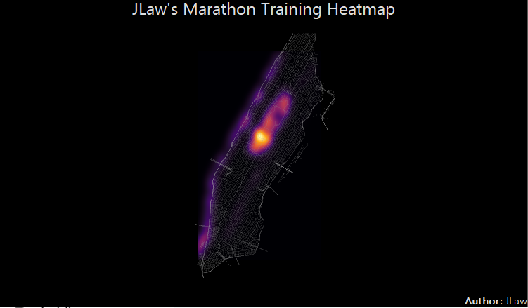
At the end of the day, my goal with this analysis is to make a cool looking heatmap of my training routes for the NYC Marathon… or at least to make a visualization that was cooler looking that my wife’s.
For those who can’t wait… this was final output:
Libraries Used
This analysis uses four main packages. Tidyverse for data manipulation, sf for modifying spatial data, tigris for getting the basemaps to plot my routes and extrafont to bring in new fonts for the plots.
library(tidyverse) # Data Manipulation
library(sf) # Manipulation Spatial Data
library(tigris) # Getting Tract and Roads Spatial Data
library(extrafont) # Better Fonts For GGPLOT
Gathering Data
If I had a GPS watch or used Strava, I could just download all my files which would contain Geo information and plot it directly. But because I do everything manually, I needed to jump through some hoops. From my MapMyRun account I was able to download:
user_workout_history.csv- Containing all of my workouts along with a column for route_id.- GPX files for each route that I had saved.
This led to the semi-painful manual process of using the first file to write down each route id that I had run, look up that route, and download the individual GPX file. Fortunately, I’m a creature of habit and and ran the same routes often, so there were only 24 to individually download.
The User Workout History File
This file was a CSV file exported from MapMyRun which contained one row for each workout I did along with meta-data such as date, time, speed, etc. However, the important column is route id which will be used to join the geo-data from the route’s GPX files.
runs <- read_csv('data/user_workout_history.csv') %>%
  # Create Route ID column
  mutate(route_id = str_extract(RouteID, '\\d+') %>% as.integer)
The Route GPX Files
As mentioned above the geocoded data for each route lives in GPX files, one for each of the 24 routes. Since I would apply the same pre-processing to each file this is a good candidate for the map_dfr function to construct the data frame.
The following code uses dir() to get a list of all the files in the directory as vectors, the keep() function trims the vector to only the GPX files, and each GPX file is then passed into read_sf to read in the geo-data. The data is subset to only two columns, and a route_id is created based on the numbers in the file name.
Finally, geo-data in sf lives in a GEOMETRY column. However, in order to get the latitudes and longitudes as individual columns I use st_coodinates to creates “X” and “Y” columns for longitude and latitude.
all_routes <- map_dfr(
  #Get all gpx files in the directory
  keep(dir('data'), ~str_detect(.x, "gpx")),
  #Read them in
  ~read_sf(paste0('data/',.x), layer = "track_points") %>%
    #keep the segment id and the geometry field
    select(track_seg_point_id, geometry) %>%
    # create a route_id based on the file
    mutate(route_id = parse_number(.x))
) %>%
  #Extract Lat and Long as Columns
  cbind(., st_coordinates(.))
After the processing the data looks like:
| track_seg_point_id | route_id | X | Y | geometry |
|---|---|---|---|---|
| 0 | 111694131 | -73.97597 | 40.77624 | POINT (-73.97597 40.77624) |
| 1 | 111694131 | -73.97555 | 40.77605 | POINT (-73.97555 40.77605) |
| 2 | 111694131 | -73.97555 | 40.77605 | POINT (-73.97555 40.77605) |
| 3 | 111694131 | -73.97546 | 40.77582 | POINT (-73.97546 40.77582) |
| 4 | 111694131 | -73.97546 | 40.77582 | POINT (-73.97546 40.77582) |
| 5 | 111694131 | -73.97552 | 40.77527 | POINT (-73.97552 40.77527) |
Combining Runs and Routes
With all the workouts in the runs data and all the routes in the all_routes data, a simple inner-join will combine them. This will duplicates routes that I ran multiple times, which in this case would be the desired behavior.
#Join Routes to Runs to Duplicate
runs_and_routes <- runs %>%
  inner_join(all_routes, by = "route_id")
Creating a map of NYC
Since the goal is to create a heatmap of the various routes I ran as part of marathon training, I need a map that contains all of the possible roads in NYC. The tigris package allows for the access to US Census TIGER shapefiles. One of the levels is “roads”, which can be downloaded using the road() function where the first parameter is state and 2nd parameter is county (New York County is Manhattan):
###Download Roads Map from Tigris
nyc <- roads("NY", "New York")
ggplot() + geom_sf(data = nyc) + ggthemes::theme_map()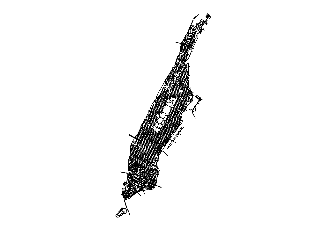
The function provides road data for all of Manhattan. However, I did not run every part of Manhattan, so it would make more sense to truncate the map to areas where I did run.
In order to do this, I first need to define a boundary box based on my routes. Given a geometry, the st_bbox() function from sf will return a “bbox” object containing the four corners of my routes.
st_bbox(runs_and_routes$geometry)## xmin ymin xmax ymax
## -74.01880 40.70806 -73.93118 40.82113However, this will not provide any padding around my running routes which will make for a worse visualization. So I will use map2_dbl to add a delta of 0.01 to the maximum values and remove a delta of -0.01 to the minimum values to slightly increase the bounding box.
### Construct Bounding Boxes and Expand Limits By A Delta
bbox <- map2_dbl(
  st_bbox(runs_and_routes$geometry),
  names(st_bbox(runs_and_routes$geometry)),
  ~if_else(str_detect(.y, 'min'), .x - .01, .x + .01)
)

bbox
## xmin ymin xmax ymax
## -74.02880 40.69806 -73.92118 40.83113With an updated bounding box, I can now crop the initial map with my bounding box using the st_crop() function. Also, in order to make the Coordinate Reference Systems the same, I use st_crs() and st_transform to make sure the NYC map is using the same coordinates as my routes.
#Set CRS for NYC to CRS for Running Routes And Crop to the Bounding Box
nyc2 <- st_transform(nyc, crs = st_crs(runs_and_routes$geometry)) %>%
  st_crop(bbox)

ggplot() + geom_sf(data = nyc2) + ggthemes::theme_map()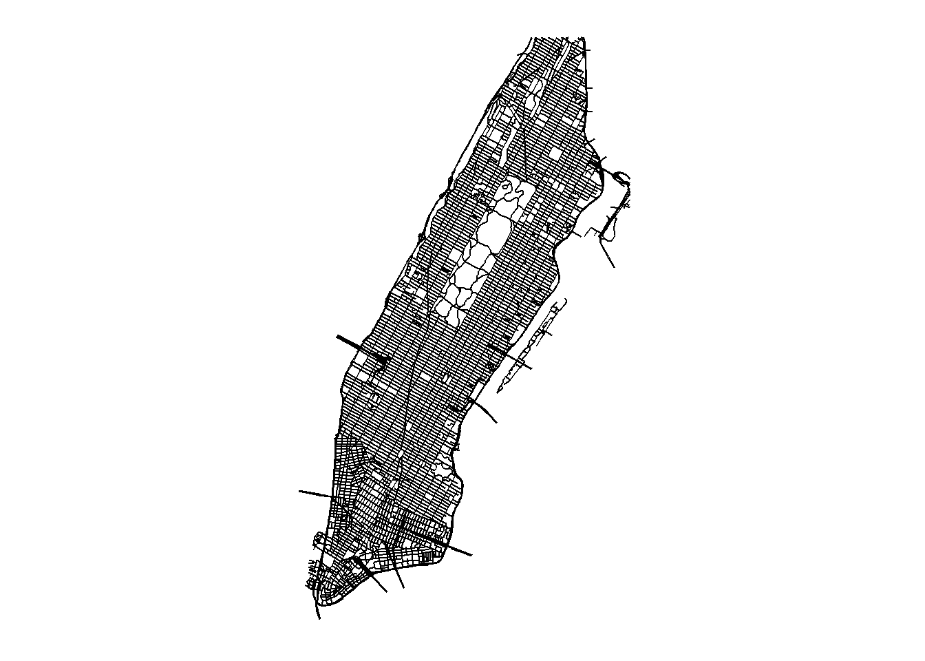
We’ve now cut off Governor’s Island from the bottom left corner as well as parts of Northern Manhattan that I never ran to.
Constructing the Heatmap
With the new basemap created and the route data in its own data frame. I can create the heatmap using stat_density2d with the route data and geom_sf with the map data. From the stat_density2d piece I pass in the routes data and set the fill value to be the count at each X and Y using the after_stat() option. The n parameter sets the number of grid points in each directions for the density.
The base map is very rectangular where it is tall but skinny. This made it difficult to add titles. To make things look better, I use ggdraw from the cowplot package to create a new drawing layer and add titles/captions to that layer.
p <- ggplot() +
  #Construct the Heatmap Portion
  stat_density2d(data = runs_and_routes,
                 aes(x = X, y = Y, fill = after_stat(count)),
                 geom = 'tile',
                 contour = F,
                 n = 1024
                 ) +
  #Draw the Map of Manhattan
  geom_sf(data = nyc2, color = '#999999', alpha = .15) +
  scale_fill_viridis_c(option = "B", guide = F) +
  ggthemes::theme_map() +
  theme(
    panel.background = element_rect(fill = 'black'),
    plot.background = element_rect(fill = 'black')
  )

cowplot::ggdraw(p) +
  labs(title = "JLaw's Marathon Training Heatmap",
       caption = "**Author**: JLaw") +
  theme(panel.background = element_rect(fill = "black"),
        plot.background = element_rect(fill = 'black'),
        plot.title = element_text(color = "#DDDDDD",
                                  family = 'Nirmala UI',
                                  #face = 'bold',
                                  size = 18),
        plot.caption = ggtext::element_markdown(color = '#DDDDDD',
                                    family = 'Calibri Light',
                                    hjust = 1,
                                    size = 12),


  )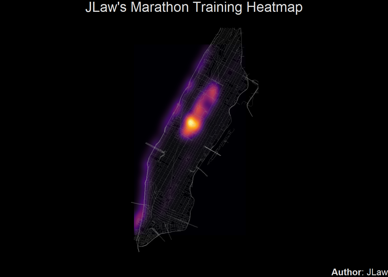
Concluding Thoughts
I’m really happy with how this came out. It also provides some information about my running habits, mainly that I ran in Central Park a lot and that you can roughly tell where I worked at the time as that area is slightly hotter. There are some parts of Manhattan that I did run but don’t show up well in the map because I might have only run there once. An exploration of how much of Manhattan did I run will be covered in a follow-up post.