What's the most successful Dancing With the Stars "Profession"? Visualizing with {gt}

Motivation
During this pandemic I’ve found a source of comfort in Dancing with the Stars (DWTS). I’ve never watched any other season before and I think a large part of starting now are:
- Lack of anything else to watch
- The rapper Nelly (and the St. Lunatics) have a near and dear place in my heart.
On the R front, I’ve wanted to mess around with the gt package for a while now but hadn’t had a great reason to. However, I had originally wanted to do a post on whether DWTS has “score inflation” throughout the season, but that wound up being more complicated than I would have liked. So instead why not answer what is the most successful type of star on Dancing with the Stars.
And on the gt front a huge shout-out to Kaustav Sen whose post on gt for the Great American Beer Festival served as a large design inspiration for this post.
The Final Output
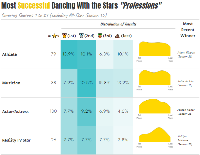
At the end of this post, the final output for the table will look like:
The Pre-Processing
Load the Libraries
The main focus of this post is on the gt package to make the table, however, other packages are used to get and work with the data.
library(rvest) #Web Scrape Wikipedia
library(tidyverse) #Data Manipulation / Plots
library(lubridate) #Date Manipulation
library(gt) #Making Fancy Tables / The Focus of This Post
library(glue) #Text Manipulation
Getting all the DWTS Contestants
In order to find the most successful star type, we need to get a list of all the contestants. Fortunately, Wikipedia has a page for every season and on those pages has a list of information about the contestants including, their name, what their known for, and their status from the season.
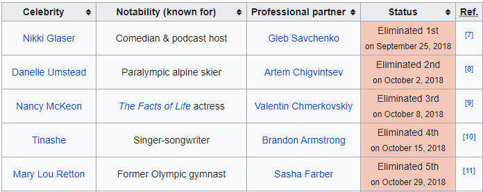
Since there are 29 completed Dancing with the Stars seasons this seems like a job for a function to iterate through each season’s Wikipedia page to extract that table. One note is that Season 15 was an all-star season so it will be excluded from this analysis Unfortunately, the contestant table isn’t always in the same place on the page, so the function will need to be a little flexible.
dwts_constants <- function(season_number, tbl_number){
  read_html(glue('https://en.wikipedia.org/wiki/Dancing_with_the_Stars_(American_season_{season_number})')) %>%
    html_nodes('table') %>%
    .[[tbl_number]] %>%
    html_table() %>%
    mutate(season = season_number) %>%
    janitor::clean_names()
}
Given a season number, and the number table on the page to extract the above function will extract and lightly clean the data. The following code will append all of the contestants on top of each other.
contestants <- dwts_constants(1, 2) %>%
  bind_rows(dwts_constants(2, 3) ) %>%
  bind_rows(dwts_constants(3, 3) ) %>%
  bind_rows(dwts_constants(4, 3) ) %>%
  bind_rows(dwts_constants(5, 2) ) %>%
  bind_rows(dwts_constants(6, 2) ) %>%
  bind_rows(dwts_constants(7, 2) ) %>%
  bind_rows(dwts_constants(8, 2) ) %>%
  bind_rows(dwts_constants(9, 2) ) %>%
  bind_rows(dwts_constants(10, 2)) %>%
  bind_rows(dwts_constants(11, 2)) %>%
  bind_rows(dwts_constants(12, 2)) %>%
  bind_rows(dwts_constants(13, 2)) %>%
  bind_rows(dwts_constants(14, 3)) %>%
  #bind_rows(dwts_constants(15, 2)) %>%  #Season 15 is an All-Star Season
  bind_rows(dwts_constants(16, 2)) %>%
  bind_rows(dwts_constants(17, 2)) %>%
  bind_rows(dwts_constants(18, 2)) %>%
  bind_rows(dwts_constants(19, 2)) %>%
  bind_rows(dwts_constants(20, 2)) %>%
  bind_rows(dwts_constants(21, 2)) %>%
  bind_rows(dwts_constants(22, 2)) %>%
  bind_rows(dwts_constants(23, 2)) %>%
  bind_rows(dwts_constants(24, 2)) %>%
  bind_rows(dwts_constants(25, 2)) %>%
  bind_rows(dwts_constants(26, 2)) %>%
  bind_rows(dwts_constants(27, 2)) %>%
  bind_rows(dwts_constants(28, 2)) %>%
  bind_rows(dwts_constants(29, 2))
Directly from this function the raw data looks like:
| celebrity | notability_known_for | professional_partner | status | season | result | professional_partner_a | ref | professional_partner_a_7 | celebrity_12_13 |
|---|---|---|---|---|---|---|---|---|---|
| Trista Sutter | The Bachelorette star | Louis Van Amstel | Eliminated 1ston June 8, 2005 | 1 | NA | NA | NA | NA | NA |
| Evander Holyfield | Heavyweight boxer | Edyta Sliwinska | Eliminated 2ndon June 15, 2005 | 1 | NA | NA | NA | NA | NA |
| Rachel Hunter | Supermodel | Jonathan Roberts | Eliminated 3rdon June 22, 2005 | 1 | NA | NA | NA | NA | NA |
Cleaning the data
Looking at the raw data there is a lot of data cleaning to be done:
- The contestant’s result shows up in two different columns (
result,status) - The
resultfield has both placing information as well as dates for when they were either eliminated or won. For example Eliminated 1st needs to be turned into placed last (depending on how many contestants there were that season) - The data contains contestants who withdrew so their place had nothing to do with their “Profession”
- The
resultfield can be cleaned up to be standardized - The
notabilityfield needs to be standardized
All of these steps are handled in the following code:
contestant_clean <- contestants %>%
  mutate(
    #Compress Fields That Have Different Names Per Season
    result = coalesce(result, status),
    #Get the dates when Eliminations / Wins Happen
    status_date = mdy(str_extract(result, "\\w+ \\d+, \\d{4}")),
    #Get the Order of Elimination
    eliminated_state = str_extract(result, "Eliminated \\d+") %>%
      str_remove('Eliminated ') %>%
      as.numeric()
  ) %>%
  # Remove Contestants that Withdraw
  filter(!str_detect(result, 'Withdrew')) %>%
  group_by(season) %>%
  # Add the number of contestants for each season
  mutate(n_contestants = n()) %>%
  ungroup() %>%
  #Overwrite Places for 1st/2nd/3rd
  mutate(
    place = case_when(
      str_detect(result, "Winner") ~ 1,
      str_detect(result, "Runner|Second") ~ 2,
      str_detect(result, "Third") ~ 3,
      str_detect(result, "Fourth") ~ 4,
      TRUE ~ n_contestants - eliminated_state + 1
    ),
    # Standardize What Contestants Are "Known For"
    known_for = case_when(
      str_detect(str_to_lower(notability_known_for),
                 'actor|actress|disney') ~ 'Actor/Actress',
      str_detect(str_to_lower(notability_known_for),
                 'singer|rapper|band|composer') ~ 'Musician',
      str_detect(str_to_lower(notability_known_for),
                 'model|miss usa') ~ 'Model',
      str_detect(str_to_lower(notability_known_for),
                 'nhl|nfl|nba|boxer|olympi|diva|tennis|soccer|football|lakers|swim|ufc|nascar|snowboard|wwe|mlb|basketball|rodeo|skier|race car|jockey|dolphins|steelers|packers|lakers|indy 500') ~ 'Athlete',
      str_detect(str_to_lower(notability_known_for),
                 'journ|anchor|host|caster|personality') ~ 'Media Personality',
      str_detect(str_to_lower(notability_known_for),
                 'bachelor|star|chef') ~ 'Reality TV Star',
      str_detect(str_to_lower(notability_known_for),
                 'comedian|magician|entertainer') ~ 'Entertainer',
      str_detect(str_to_lower(notability_known_for),
                 'owner|co-founder|business|designer') ~ 'Businessperson',
      TRUE ~ "Other"
    )
  ) %>%
  # Fix Celebrity Column for Season 29
  mutate(celebrity = if_else(is.na(celebrity), celebrity_12_13, celebrity)) %>%
  # Remove Unneeded Columns
  select(-contains('professional'), -ref, -status,
         -eliminated_state, -celebrity_12_13) %>%
  #Want Scores to be between 0 and 1 where 1 is Last Place and 0 is first place.
  mutate(scaled_place = (place-1)/(n_contestants-1))
The scaled_place variable will be used to create a standardized density plot by putting each season on a 1 (Last Place) to 0 (1st Place) scale regardless of the number of contestants in the season. The cleaned data now looks like:
| celebrity | notability_known_for | season | result | status_date | n_contestants | place | known_for | scaled_place |
|---|---|---|---|---|---|---|---|---|
| Trista Sutter | The Bachelorette star | 1 | Eliminated 1ston June 8, 2005 | 2005-06-08 | 6 | 6 | Reality TV Star | 1.0 |
| Evander Holyfield | Heavyweight boxer | 1 | Eliminated 2ndon June 15, 2005 | 2005-06-15 | 6 | 5 | Athlete | 0.8 |
| Rachel Hunter | Supermodel | 1 | Eliminated 3rdon June 22, 2005 | 2005-06-22 | 6 | 4 | Model | 0.6 |
| Joey McIntyre | New Kids on the Block singer | 1 | Third placeon June 29, 2005 | 2005-06-29 | 6 | 3 | Musician | 0.4 |
| John O’Hurley | Actor & game show host | 1 | Runner-upon July 6, 2005 | 2005-07-06 | 6 | 2 | Actor/Actress | 0.2 |
Using Regular Expressions, I’ve collapsed 237 different levels into 9 which are:
| Profession | Examples |
|---|---|
| Actor/Actress | Zendaya, Alexa PenaVega, Amber Riley |
| Athlete | Jamie Anderson, Antonio Brown, Martina Navratilova |
| Businessperson | Steve Wozniak, Robert Herjavec, Mark Cuban |
| Entertainer | Penn Jillette, Marie Osmond, Margaret Cho |
| Media Personality | Jerry Springer, Bobby Bones, Giselle Fernandez |
| Model | Bonner Bolton, Shandi Finnessey, Sailor Brinkley-Cook |
| Musician | Joey McIntyre, Gavin DeGraw, Nick Carter |
| Other | Sean Spicer, Buzz Aldrin, Noah Galloway |
| Reality TV Star | The Situation, Lisa Vanderpump, Terra Jolé |
Constructing The Table
Organizing the Data
For the table, the information we want is for each “Profession”:
- How many contestants were there?
- What percentages came in 1st, 2nd, 3rd, and Last?
Some quick dplyr magic will allow us to collapse the list of contestants into the structure we want. We’ll also set the order of the table by the descending percentage of first place wins by “profession”.
contestant_summary <- contestant_clean %>%
  group_by(known_for) %>%
  summarize(
    num_stars = n(),
    pct_1st_place = sum(place == 1)/n(),
    pct_2nd_place = sum(place == 2)/n(),
    pct_3rd_place = sum(place == 3)/n(),
    pct_last_place = sum(n_contestants == place) / n()
  ) %>%
  arrange(-pct_1st_place)
Using {gt} to Build the Table
Now onto actually constructing the table with gt. The gt package provides a grammar for tables similar to what ggplot2 does for charts. The package provides this visualization to show the different parts of a table:

Step 1: The basic construction
The most basic construction of a table is done by using the gt() function.
(g1 <- gt(contestant_summary))| known_for | num_stars | pct_1st_place | pct_2nd_place | pct_3rd_place | pct_last_place |
|---|---|---|---|---|---|
| Athlete | 79 | 0.13924051 | 0.10126582 | 0.06329114 | 0.10126582 |
| Musician | 38 | 0.07894737 | 0.10526316 | 0.15789474 | 0.13157895 |
| Actor/Actress | 130 | 0.07692308 | 0.09230769 | 0.06923077 | 0.04615385 |
| Reality TV Star | 26 | 0.07692308 | 0.07692308 | 0.07692308 | 0.03846154 |
| Model | 14 | 0.07142857 | 0.07142857 | 0.00000000 | 0.07142857 |
| Media Personality | 21 | 0.04761905 | 0.04761905 | 0.04761905 | 0.23809524 |
| Businessperson | 5 | 0.00000000 | 0.00000000 | 0.00000000 | 0.20000000 |
| Entertainer | 5 | 0.00000000 | 0.00000000 | 0.20000000 | 0.40000000 |
| Other | 9 | 0.00000000 | 0.00000000 | 0.44444444 | 0.00000000 |
When I said basic, I meant basic.
Step 2: Adding Titles and Subtitles
The tab_header() function allows alterations to the header of the table. The title and subtitle arguments create the title and subtitle respectively. A nice feature of gt is the html() function will allows the use of HTML and CSS to style these titles. There is also a md() function that allows for markdown rendering.
(g2 <- g1 %>%
  tab_header(
    title = html('Most <span style="color:#F2CB05">Successful</span> Dancing With the Stars <i>"Professions"</i>'),
    subtitle = html(
      "<span style = 'color: grey'>Covering Seasons 1 to 29 (excluding All-Star Season 15)</span>"
    )
))| Most Successful Dancing With the Stars "Professions" | |||||
|---|---|---|---|---|---|
| Covering Seasons 1 to 29 (excluding All-Star Season 15) | |||||
| known_for | num_stars | pct_1st_place | pct_2nd_place | pct_3rd_place | pct_last_place |
| Athlete | 79 | 0.13924051 | 0.10126582 | 0.06329114 | 0.10126582 |
| Musician | 38 | 0.07894737 | 0.10526316 | 0.15789474 | 0.13157895 |
| Actor/Actress | 130 | 0.07692308 | 0.09230769 | 0.06923077 | 0.04615385 |
| Reality TV Star | 26 | 0.07692308 | 0.07692308 | 0.07692308 | 0.03846154 |
| Model | 14 | 0.07142857 | 0.07142857 | 0.00000000 | 0.07142857 |
| Media Personality | 21 | 0.04761905 | 0.04761905 | 0.04761905 | 0.23809524 |
| Businessperson | 5 | 0.00000000 | 0.00000000 | 0.00000000 | 0.20000000 |
| Entertainer | 5 | 0.00000000 | 0.00000000 | 0.20000000 | 0.40000000 |
| Other | 9 | 0.00000000 | 0.00000000 | 0.44444444 | 0.00000000 |
Step 3: Adding More Style to the Title
The tab_style() function adds various formatting to the table rows and cells. The style section of the arguments tells gt what the style will be and the location argument says where that style should be applied.
The google_font() function allows access to all the fonts on the Google Fonts site.
In this step I’m making the title left-justified, size XX-Large, and using the Anton font.
(g3 <- g2 %>%
  tab_style(
    style = cell_text(
      font = google_font("Anton"),
      align = "left",
      size = "xx-large"
    ),
    locations = cells_title("title")
  )
)| Most Successful Dancing With the Stars "Professions" | |||||
|---|---|---|---|---|---|
| Covering Seasons 1 to 29 (excluding All-Star Season 15) | |||||
| known_for | num_stars | pct_1st_place | pct_2nd_place | pct_3rd_place | pct_last_place |
| Athlete | 79 | 0.13924051 | 0.10126582 | 0.06329114 | 0.10126582 |
| Musician | 38 | 0.07894737 | 0.10526316 | 0.15789474 | 0.13157895 |
| Actor/Actress | 130 | 0.07692308 | 0.09230769 | 0.06923077 | 0.04615385 |
| Reality TV Star | 26 | 0.07692308 | 0.07692308 | 0.07692308 | 0.03846154 |
| Model | 14 | 0.07142857 | 0.07142857 | 0.00000000 | 0.07142857 |
| Media Personality | 21 | 0.04761905 | 0.04761905 | 0.04761905 | 0.23809524 |
| Businessperson | 5 | 0.00000000 | 0.00000000 | 0.00000000 | 0.20000000 |
| Entertainer | 5 | 0.00000000 | 0.00000000 | 0.20000000 | 0.40000000 |
| Other | 9 | 0.00000000 | 0.00000000 | 0.44444444 | 0.00000000 |
Step 4: Add Styling to the Subtitles
Similar to step 3, this step applies formatting to the subtitle
(g4 <- g3 %>%
  tab_style(
    style = cell_text(
      font = google_font("Caveat"),
      align = "left",
      size = "x-large"
    ),
    locations = cells_title("subtitle")
  )
)| Most Successful Dancing With the Stars "Professions" | |||||
|---|---|---|---|---|---|
| Covering Seasons 1 to 29 (excluding All-Star Season 15) | |||||
| known_for | num_stars | pct_1st_place | pct_2nd_place | pct_3rd_place | pct_last_place |
| Athlete | 79 | 0.13924051 | 0.10126582 | 0.06329114 | 0.10126582 |
| Musician | 38 | 0.07894737 | 0.10526316 | 0.15789474 | 0.13157895 |
| Actor/Actress | 130 | 0.07692308 | 0.09230769 | 0.06923077 | 0.04615385 |
| Reality TV Star | 26 | 0.07692308 | 0.07692308 | 0.07692308 | 0.03846154 |
| Model | 14 | 0.07142857 | 0.07142857 | 0.00000000 | 0.07142857 |
| Media Personality | 21 | 0.04761905 | 0.04761905 | 0.04761905 | 0.23809524 |
| Businessperson | 5 | 0.00000000 | 0.00000000 | 0.00000000 | 0.20000000 |
| Entertainer | 5 | 0.00000000 | 0.00000000 | 0.20000000 | 0.40000000 |
| Other | 9 | 0.00000000 | 0.00000000 | 0.44444444 | 0.00000000 |
Step 5: Adding a Spanner Column
A spanner column is a column header that is merged across a number of different columns. It is added with the tab_spanner() function:
(g5 <- g4 %>%
  tab_spanner(
    label = "Distribution of Results",
    columns = 3:6
  )
)| Most Successful Dancing With the Stars "Professions" | |||||
|---|---|---|---|---|---|
| Covering Seasons 1 to 29 (excluding All-Star Season 15) | |||||
| known_for | num_stars | Distribution of Results | |||
| pct_1st_place | pct_2nd_place | pct_3rd_place | pct_last_place | ||
| Athlete | 79 | 0.13924051 | 0.10126582 | 0.06329114 | 0.10126582 |
| Musician | 38 | 0.07894737 | 0.10526316 | 0.15789474 | 0.13157895 |
| Actor/Actress | 130 | 0.07692308 | 0.09230769 | 0.06923077 | 0.04615385 |
| Reality TV Star | 26 | 0.07692308 | 0.07692308 | 0.07692308 | 0.03846154 |
| Model | 14 | 0.07142857 | 0.07142857 | 0.00000000 | 0.07142857 |
| Media Personality | 21 | 0.04761905 | 0.04761905 | 0.04761905 | 0.23809524 |
| Businessperson | 5 | 0.00000000 | 0.00000000 | 0.00000000 | 0.20000000 |
| Entertainer | 5 | 0.00000000 | 0.00000000 | 0.20000000 | 0.40000000 |
| Other | 9 | 0.00000000 | 0.00000000 | 0.44444444 | 0.00000000 |
Step 6: Styling the Spanner
Similar to the title and subtitle, we can use tab_style() to apply specific styles to the spanner via the cells_column_spanners() function.
(g6 <- g5 %>%
  tab_style(
    style = cell_text(
      font = google_font("Courgette"),
      size = "medium",
      weight = "bold"
    ),
    locations = cells_column_spanners("Distribution of Results")
  )
)| Most Successful Dancing With the Stars "Professions" | |||||
|---|---|---|---|---|---|
| Covering Seasons 1 to 29 (excluding All-Star Season 15) | |||||
| known_for | num_stars | Distribution of Results | |||
| pct_1st_place | pct_2nd_place | pct_3rd_place | pct_last_place | ||
| Athlete | 79 | 0.13924051 | 0.10126582 | 0.06329114 | 0.10126582 |
| Musician | 38 | 0.07894737 | 0.10526316 | 0.15789474 | 0.13157895 |
| Actor/Actress | 130 | 0.07692308 | 0.09230769 | 0.06923077 | 0.04615385 |
| Reality TV Star | 26 | 0.07692308 | 0.07692308 | 0.07692308 | 0.03846154 |
| Model | 14 | 0.07142857 | 0.07142857 | 0.00000000 | 0.07142857 |
| Media Personality | 21 | 0.04761905 | 0.04761905 | 0.04761905 | 0.23809524 |
| Businessperson | 5 | 0.00000000 | 0.00000000 | 0.00000000 | 0.20000000 |
| Entertainer | 5 | 0.00000000 | 0.00000000 | 0.20000000 | 0.40000000 |
| Other | 9 | 0.00000000 | 0.00000000 | 0.44444444 | 0.00000000 |
Step 7: Style the Column Headers and the Profession Column
You can apply the same style to different parts of the table by using a list() for the locations argument. Here the style is being applied to all column labels (cells_column_labels(everything())) and to the values in the first column (cells_body(columns = 1)).
(g7 <- g6 %>%
  tab_style(
    style = cell_text(
      font = google_font("Secular One"),
      size = "large"
    ),
    locations = list(
      cells_column_labels(everything()),
      cells_body(columns = 1)
    )
  )
)| Most Successful Dancing With the Stars "Professions" | |||||
|---|---|---|---|---|---|
| Covering Seasons 1 to 29 (excluding All-Star Season 15) | |||||
| known_for | num_stars | Distribution of Results | |||
| pct_1st_place | pct_2nd_place | pct_3rd_place | pct_last_place | ||
| Athlete | 79 | 0.13924051 | 0.10126582 | 0.06329114 | 0.10126582 |
| Musician | 38 | 0.07894737 | 0.10526316 | 0.15789474 | 0.13157895 |
| Actor/Actress | 130 | 0.07692308 | 0.09230769 | 0.06923077 | 0.04615385 |
| Reality TV Star | 26 | 0.07692308 | 0.07692308 | 0.07692308 | 0.03846154 |
| Model | 14 | 0.07142857 | 0.07142857 | 0.00000000 | 0.07142857 |
| Media Personality | 21 | 0.04761905 | 0.04761905 | 0.04761905 | 0.23809524 |
| Businessperson | 5 | 0.00000000 | 0.00000000 | 0.00000000 | 0.20000000 |
| Entertainer | 5 | 0.00000000 | 0.00000000 | 0.20000000 | 0.40000000 |
| Other | 9 | 0.00000000 | 0.00000000 | 0.44444444 | 0.00000000 |
Step 8: Styling the cells
Applying a center alignment to the 2nd through 6th columns.
(g8 <- g7 %>%
  tab_style(
    style = cell_text(
      font = google_font("Spartan"),
      size = "medium",
      align = 'center'
    ),
    locations = cells_body(columns = 2:6)
  )
)| Most Successful Dancing With the Stars "Professions" | |||||
|---|---|---|---|---|---|
| Covering Seasons 1 to 29 (excluding All-Star Season 15) | |||||
| known_for | num_stars | Distribution of Results | |||
| pct_1st_place | pct_2nd_place | pct_3rd_place | pct_last_place | ||
| Athlete | 79 | 0.13924051 | 0.10126582 | 0.06329114 | 0.10126582 |
| Musician | 38 | 0.07894737 | 0.10526316 | 0.15789474 | 0.13157895 |
| Actor/Actress | 130 | 0.07692308 | 0.09230769 | 0.06923077 | 0.04615385 |
| Reality TV Star | 26 | 0.07692308 | 0.07692308 | 0.07692308 | 0.03846154 |
| Model | 14 | 0.07142857 | 0.07142857 | 0.00000000 | 0.07142857 |
| Media Personality | 21 | 0.04761905 | 0.04761905 | 0.04761905 | 0.23809524 |
| Businessperson | 5 | 0.00000000 | 0.00000000 | 0.00000000 | 0.20000000 |
| Entertainer | 5 | 0.00000000 | 0.00000000 | 0.20000000 | 0.40000000 |
| Other | 9 | 0.00000000 | 0.00000000 | 0.44444444 | 0.00000000 |
Step 9: Turn Cell Decimals to Percentages
There are a number of fmt_* functions to handle formatting for values. The fmt_percent function will apply a percent format to all the columns beginning with “pct_”. While this is the first instance of using tidyselect syntax for telling gt what columns to use, the package can take names, column numbers, or tidyselect.
(g9 <- g8 %>%
  fmt_percent(
    columns = starts_with('pct'),
    decimals = 1,
    drop_trailing_zeros = TRUE
  )
)| Most Successful Dancing With the Stars "Professions" | |||||
|---|---|---|---|---|---|
| Covering Seasons 1 to 29 (excluding All-Star Season 15) | |||||
| known_for | num_stars | Distribution of Results | |||
| pct_1st_place | pct_2nd_place | pct_3rd_place | pct_last_place | ||
| Athlete | 79 | 13.9% | 10.1% | 6.3% | 10.1% |
| Musician | 38 | 7.9% | 10.5% | 15.8% | 13.2% |
| Actor/Actress | 130 | 7.7% | 9.2% | 6.9% | 4.6% |
| Reality TV Star | 26 | 7.7% | 7.7% | 7.7% | 3.8% |
| Model | 14 | 7.1% | 7.1% | 0% | 7.1% |
| Media Personality | 21 | 4.8% | 4.8% | 4.8% | 23.8% |
| Businessperson | 5 | 0% | 0% | 0% | 20% |
| Entertainer | 5 | 0% | 0% | 20% | 40% |
| Other | 9 | 0% | 0% | 44.4% | 0% |
Step 10: Have some fun by turning column headers into emojis
Like other markdown text in R gt can also support emojis! Here we can add in medals for 1st, 2nd, and 3rd…. and a personal favorite emoji to represent last. Emojis can be added into markdown through the emo::ji() function.
(g10 <- g9 %>%
  cols_label(
    known_for = "",
    num_stars = paste0("# ",emo::ji('star'), "s"),
    pct_1st_place = paste0(emo::ji("1st_place_medal"), "(1st)"),
    pct_2nd_place = paste0(emo::ji("2nd_place_medal"), "(2nd)"),
    pct_3rd_place = paste0(emo::ji("3rd_place_medal"), "(3rd)"),
    pct_last_place = paste0(emo::ji("poo"), " (last)")
  )
)| Most Successful Dancing With the Stars "Professions" | |||||
|---|---|---|---|---|---|
| Covering Seasons 1 to 29 (excluding All-Star Season 15) | |||||
| # ⭐s | Distribution of Results | ||||
| 🥇(1st) | 🥈(2nd) | 🥉(3rd) | 💩 (last) | ||
| Athlete | 79 | 13.9% | 10.1% | 6.3% | 10.1% |
| Musician | 38 | 7.9% | 10.5% | 15.8% | 13.2% |
| Actor/Actress | 130 | 7.7% | 9.2% | 6.9% | 4.6% |
| Reality TV Star | 26 | 7.7% | 7.7% | 7.7% | 3.8% |
| Model | 14 | 7.1% | 7.1% | 0% | 7.1% |
| Media Personality | 21 | 4.8% | 4.8% | 4.8% | 23.8% |
| Businessperson | 5 | 0% | 0% | 0% | 20% |
| Entertainer | 5 | 0% | 0% | 20% | 40% |
| Other | 9 | 0% | 0% | 44.4% | 0% |
Step 11: Add a source and do some formatting
There a couple things going on in this step:
- I’m adding a source line with
tab_source_note()and usingmd()to allow me to use markdown style formatting. - I’m using
tab_options()to remove the top border from the table and shrink the gaps between the rows in the table. - I’m using
cols_width()to tellgtto make the first column 200px wide
(g11 <- g10 %>%
  tab_source_note(md("**Data:** DWTS Wikipedia Articles | **Table Author:** JLaw")) %>%
  tab_options(
    table.border.top.color = "white",
    data_row.padding = px(0),
  ) %>%
  cols_width(
    1 ~ px(200),
  )
)| Most Successful Dancing With the Stars "Professions" | |||||
|---|---|---|---|---|---|
| Covering Seasons 1 to 29 (excluding All-Star Season 15) | |||||
| # ⭐s | Distribution of Results | ||||
| 🥇(1st) | 🥈(2nd) | 🥉(3rd) | 💩 (last) | ||
| Athlete | 79 | 13.9% | 10.1% | 6.3% | 10.1% |
| Musician | 38 | 7.9% | 10.5% | 15.8% | 13.2% |
| Actor/Actress | 130 | 7.7% | 9.2% | 6.9% | 4.6% |
| Reality TV Star | 26 | 7.7% | 7.7% | 7.7% | 3.8% |
| Model | 14 | 7.1% | 7.1% | 0% | 7.1% |
| Media Personality | 21 | 4.8% | 4.8% | 4.8% | 23.8% |
| Businessperson | 5 | 0% | 0% | 0% | 20% |
| Entertainer | 5 | 0% | 0% | 20% | 40% |
| Other | 9 | 0% | 0% | 44.4% | 0% |
| Data: DWTS Wikipedia Articles | Table Author: JLaw | |||||
Step 12: Adding a Color Scale for the % Columns
The data_color function allows for doing conditional formatting based on the values in the columns. The columns argument allows to specific which colors should receive the formatting. The colors argument defines the palette. And the apply_to argument can take the values of “fill” to fill the background or “text” to change the color of the text.
(g12 <- g11 %>%
  data_color(
    columns = vars(pct_1st_place, pct_2nd_place, pct_3rd_place, pct_last_place),
    colors = scales::col_numeric(
      palette = c("white", "#3fc1c9"),
      #F2CB05 = Gold COlor
      domain = NULL
    ),
    apply_to = "fill",
  )
)| Most Successful Dancing With the Stars "Professions" | |||||
|---|---|---|---|---|---|
| Covering Seasons 1 to 29 (excluding All-Star Season 15) | |||||
| # ⭐s | Distribution of Results | ||||
| 🥇(1st) | 🥈(2nd) | 🥉(3rd) | 💩 (last) | ||
| Athlete | 79 | 13.9% | 10.1% | 6.3% | 10.1% |
| Musician | 38 | 7.9% | 10.5% | 15.8% | 13.2% |
| Actor/Actress | 130 | 7.7% | 9.2% | 6.9% | 4.6% |
| Reality TV Star | 26 | 7.7% | 7.7% | 7.7% | 3.8% |
| Model | 14 | 7.1% | 7.1% | 0% | 7.1% |
| Media Personality | 21 | 4.8% | 4.8% | 4.8% | 23.8% |
| Businessperson | 5 | 0% | 0% | 0% | 20% |
| Entertainer | 5 | 0% | 0% | 20% | 40% |
| Other | 9 | 0% | 0% | 44.4% | 0% |
| Data: DWTS Wikipedia Articles | Table Author: JLaw | |||||
This looks pretty good… but we can do better!!!
Turning it up to 11 by adding in Density Plots
In order to add in ggplots into a row in the table we need to:
- Build a function to create the plot for each row of the table
- Use
purrr:map()to add the plot as a list-column to the table - Use
gt::text_transformto insert the image into the table
NOTE: Since this required making a new data set much of the gt code is repeating the first section but is provided in its entirely for completeness.
Writing the function to build the chart
For the function I want it to take a “profession” and return a density part using the scaled_place variable defined at the top. The function takes in a profession label and a dataset and returns a density plot.
plot_dens <- function(profession, data) {

  plot_data <-
    data %>%
    filter(known_for == {{ profession }})

  plot <-
    plot_data %>%
    ggplot(aes(x = scaled_place)) +
    geom_density(aes(y = ..scaled..), fill = 'gold') +
    annotate("text", x = 0, y = -.05,
             label = "1st\nPlace", size = 10, color = "grey40", vjust = 1) +
    annotate("text", x = 1, y = -.05,
             label = "Last\nPlace", size = 10, color = "grey40", vjust = 1) +
    coord_cartesian(
      xlim = c(-.1, 1.1),
      ylim = c(-.7, NA)
    ) +
    theme_void()

  plot

}
Adding the plots into the data set
The main part of this step is using the map() function to iterate through the professions and use them as input into the function defined above. The column plots is a list-column containing all the ggplot information.
The left join is because I want to add in a column for the most recent winner in each category.
contestant_summary_with_graph <- contestant_summary %>%
  mutate(plots = purrr::map(contestant_summary$known_for %>% unique,
                            plot_dens, data = contestant_clean)) %>%
  left_join(
  ###Add in Recent Winner Images
  contestant_clean %>%
    filter(place == 1) %>%
    group_by(known_for) %>%
    slice_max(season, n = 1) %>%
    select(celebrity, season, known_for) %>%
    ungroup() %>%
    transmute(
      known_for,
      lbl = paste0(celebrity,' (Season ',season,")")
    )
  )
Creating the Final Table
In order to turn the plots into columns the text_transform() function is used to take the plots column and run a function that calls ggplot_image with certain height and aspect ratio parameters on each row in the table.
text_transform(
    locations = cells_body(vars(plots)),
    fn = function(x) {
      map(contestant_summary_with_graph$plots, ggplot_image,
          height = px(120), aspect_ratio = 1.5)
    }
  )
Now we can put it all together. Besides adding in the plots, there’s a few steps to format the Most Recent Winner cell. But nothing that hasn’t been covered earlier.
#Base Table
gt(contestant_summary_with_graph) %>%
  #Add Titles
  tab_header(
    title = html('Most <span style="color:#F2CB05">Successful</span> Dancing With the Stars <i>"Professions"</i>'),
    subtitle = html(
      "<span style = 'color: grey'>Covering Seasons 1 to 29 (excluding All-Star Season 15)</span>"
    )
  ) %>%
  #Format Title
  tab_style(
    style = cell_text(
      font = google_font("Anton"),
      align = "left",
      size = "xx-large"
    ),
    locations = cells_title("title")
  ) %>%
  #Format Subtitle
  tab_style(
    style = cell_text(
      font = google_font("Caveat"),
      align = "left",
      size = "x-large"
    ),
    locations = cells_title("subtitle")
  )  %>%
  #Adding Spanning Column
  tab_spanner(
    label = "Distribution of Results",
    columns = 3:7
  ) %>%
  #Style The Spanner Column
  tab_style(
    style = cell_text(
      font = google_font("Courgette"),
      size = "medium",
      weight = "bold"
    ),
    locations = cells_column_spanners("Distribution of Results")
  ) %>%
  #Style the Column Labels and Profession Column
  tab_style(
    style = cell_text(
      font = google_font("Secular One"),
      size = "large"
    ),
    locations = list(
      cells_column_labels(everything()),
      cells_body(columns = 1)
    )
  )  %>%
  #Style the Cells
  tab_style(
    style = cell_text(
      font = google_font("Spartan"),
      size = "medium",
      align = 'center'
    ),
    locations = cells_body(columns = 2:6)
  ) %>%
  #Format Cells to %s
  fmt_percent(
    columns = starts_with('pct'),
    decimals = 1,
    drop_trailing_zeros = TRUE
  ) %>%
  #Turn Headers to Emojis
  cols_label(
    known_for = "",
    num_stars = paste0("# ",emo::ji('star'), "s"),
    pct_1st_place = paste0(emo::ji("1st_place_medal"), "(1st)"),
    pct_2nd_place = paste0(emo::ji("2nd_place_medal"), "(2nd)"),
    pct_3rd_place = paste0(emo::ji("3rd_place_medal"), "(3rd)"),
    pct_last_place = paste0(emo::ji("poo"), " (last)"),
    plots = "",
    lbl = "Most Recent Winner"
  ) %>%
  ###Add in Source and Doing Some Minor Formatting
  tab_source_note(md("**Data:** DWTS Wikipedia Articles | **Table Author:** JLaw")) %>%
  tab_options(
    table.border.top.color = "white",
    data_row.padding = px(0),
  ) %>%
  cols_width(
    1 ~ px(200)
  ) %>%
###Add a Color Scale for 1st Place
  data_color(
    columns = vars(pct_1st_place, pct_2nd_place, pct_3rd_place, pct_last_place),
    colors = scales::col_numeric(
      palette = c("white", "#3fc1c9"),
      #F2CB05 = Gold COlor
      domain = NULL
    ),
    apply_to = "fill",
  ) %>%
  ######################NEW THINGS START HERE#########################
  # Add In Density Plots (NEW)
  text_transform(
    locations = cells_body(vars(plots)),
    fn = function(x) {
      map(contestant_summary_with_graph$plots, ggplot_image,
          height = px(120), aspect_ratio = 1.5)
    }
  ) %>%
  text_transform(
    locations = cells_body(vars(lbl)),
    fn = function(x){
      if_else(!is.na(x), str_replace_all(x, " \\(", "<br> \\("), "")
    }
  ) %>%
  tab_style(
    style = cell_text(
      style = 'italic',
      size = px(13),
      v_align = 'middle',
      align = 'left'
    ),
    locations = cells_body(columns = vars(lbl))
  ) %>%
  cols_width(
    8 ~ px(100)
)| Most Successful Dancing With the Stars "Professions" | |||||||
|---|---|---|---|---|---|---|---|
| Covering Seasons 1 to 29 (excluding All-Star Season 15) | |||||||
| # ⭐s | Distribution of Results | Most Recent Winner | |||||
| 🥇(1st) | 🥈(2nd) | 🥉(3rd) | 💩 (last) | ||||
| Athlete | 79 | 13.9% | 10.1% | 6.3% | 10.1% |  |
Adam Rippon (Season 26) |
| Musician | 38 | 7.9% | 10.5% | 15.8% | 13.2% |  |
Kellie Pickler (Season 16) |
| Actor/Actress | 130 | 7.7% | 9.2% | 6.9% | 4.6% |  |
Jordan Fisher (Season 25) |
| Reality TV Star | 26 | 7.7% | 7.7% | 7.7% | 3.8% |  |
Kaitlyn Bristowe (Season 29) |
| Model | 14 | 7.1% | 7.1% | 0% | 7.1% |  |
Brooke Burke (Season 7) |
| Media Personality | 21 | 4.8% | 4.8% | 4.8% | 23.8% |  |
Bobby Bones (Season 27) |
| Businessperson | 5 | 0% | 0% | 0% | 20% |  |
|
| Entertainer | 5 | 0% | 0% | 20% | 40% |  |
|
| Other | 9 | 0% | 0% | 44.4% | 0% |  |
|
| Data: DWTS Wikipedia Articles | Table Author: JLaw | |||||||
So what is the most successful “profession” in DWTS?
Seems pretty clearly to be the athletes as close to 14% of the Athletes have wound up winning. On the other end of the spectrum, the Media Personalities have faired less well with the lowest winning percentage of a group with 10+ stars and nearly 1 in 4 coming in last place… Reality TV Stars, while in the middle of the pack has been surging with ex-Bachelorettes winning the last two seasons (28 and 29).