A Racing Barplot of Top US Baby Names 1880-2018
A few month’s back Mrs. JLaw and I were discussing baby names (purely for academic purposes) and it got me thinking about how have popular names changed over time. It was a particular interest to me as someone who had a name that was somewhat popular for a while and has since fallen out of fashion.
This also provided me an opportunity to try out one of those ‘racing barplots’ that have been popping up all over the place. Also, while I’ve used the gganimate package a number of times, I constantly forget the syntax. And since this site is as much for me (probably moreso) than anyone else, this will be a good reference in case I try to do this again.
On to the project….
Fortunately, I know that baby name data is easily available as the Social Security Administration website. And while I don’t reminder how I found the flat files for all years it is available as a ZIP file containing 139 .txt files, containing popular boys and girls names for each year. However, I don’t really want to deal with downloading and unzipping files, so I’m going to try to query the SSA site directly.
Loading Some Libraries
To do this project, I’ll use:
httr- To construct the POST command to get the SSA to return a webpage with the data I wantrvest- To scrape the table of popular name data from the content returned from thehttrrequesttidyversemeta-package - for combining the data from each request (purrr), data manipulation (dplyr), and visualization (ggplot2)gganimate- to animate the ggplot2 plots and make them look super coolscales- To make the count of baby names in the chart appear prettier (comma-formatted)
library(tidyverse)
library(gganimate)
library(scales)
library(httr)
library(rvest)
Reading the Data
As mentioned before, the data is available as a series of .txt files from the SSA. When I originally did this, I downloaded and extracted the ZIP file, but as I’m redoing this for the post, I’d rather have a solution that is entirely self-contained so I’m going to try to use httr to actually query the SSA data.
So how to actually get the data from the website?
From the Baby Names By Birth Year section, I can input the birth year, how many names I want, and whether I want counts or percentages.
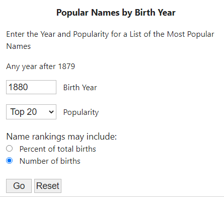
When I click go, I wind up at https://www.ssa.gov/cgi-bin/popularnames.cgi with my desired results in a table. Using Google Chrome’s Network Inspector I can see that I sent a POST request with three parameters (year, top, and number):

Now that I know what I need to send, I can create a function in purrr to request each year and stack each response on top of each other using map_dfr. For the inputs, I know that I want all available years (which I know are 1880 through 2018) and I only need the top 10 (so top = 10) and I want counts rather than percentages (number = “n”)
babynames <- map_dfr(
  1880:2018, #Inputs to My Function
  #Define Function to Apply for Each Year
  function(year){
    #Construct POST Command
    POST(
      #Where to Send the Request
      url = "https://www.ssa.gov/cgi-bin/popularnames.cgi",
      #What to Send the Requests (my three parameters)
      body = paste0("year=",year,"&top=10&number=n")
    ) %>%
    #Extract the Content from the Request Response
    content("parsed") %>%
    #Extract All The Tables
    html_nodes('table') %>%
    #Only Keep the 3rd Table (done through some guess and check)
    .[[3]] %>%
    #Store the Table Data as a data.frame
    html_table() %>%
    #Add a column to the data frame for year
    mutate(
      year = year
    )
  }
)
My expectation for this data is that there would be 139 distinct values for year and 1390 rows in the data. And in fact there are 139 distinct years (😍) and 1529 rows (😡).
So what’s going on… Let’s look at the year 1880.
| Rank | Male name | Number of males | Female name | Number of females | year |
|---|---|---|---|---|---|
| 1 | John | 9,655 | Mary | 7,065 | 1880 |
| 2 | William | 9,532 | Anna | 2,604 | 1880 |
| 3 | James | 5,927 | Emma | 2,003 | 1880 |
| 4 | Charles | 5,348 | Elizabeth | 1,939 | 1880 |
| 5 | George | 5,126 | Minnie | 1,746 | 1880 |
| 6 | Frank | 3,242 | Margaret | 1,578 | 1880 |
| 7 | Joseph | 2,632 | Ida | 1,472 | 1880 |
| 8 | Thomas | 2,534 | Alice | 1,414 | 1880 |
| 9 | Henry | 2,444 | Bertha | 1,320 | 1880 |
| 10 | Robert | 2,415 | Sarah | 1,288 | 1880 |
| Note: Rank 1 is the most popular, | |||||
| rank 2 is the next most popular, and so forth. All names are from Social Security card applications | |||||
| for births that occurred in the United States. Note: Rank 1 is the most popular, | |||||
| rank 2 is the next most popular, and so forth. All names are from Social Security card applications | |||||
| for births that occurred in the United States. Note: Rank 1 is the most popular, | |||||
| rank 2 is the next most popular, and so forth. All names are from Social Security card applications | |||||
| for births that occurred in the United States. Note: Rank 1 is the most popular, | |||||
| rank 2 is the next most popular, and so forth. All names are from Social Security card applications | |||||
| for births that occurred in the United States. Note: Rank 1 is the most popular, | |||||
| rank 2 is the next most popular, and so forth. All names are from Social Security card applications | |||||
| for births that occurred in the United States. 1880 |
Cleaning the Data
We were expected 10 rows but we got 11 because of a footnote at the bottom of the table. I could go fix the data pulling step to explicitly only get the Top 10 rows but there are a bunch of other data cleaning steps to do, so may as well do everything at once. In this step I’m going to:
- Remove that pesky footer row
- Turn the Table from Wide Format to Long Format (so genders are on top of each other)
- Convert the Counts to Numeric
babynames_clean <- babynames %>%
  #Remove the Note row by filter rows where the Rank column has the string "Note"
  filter(!str_detect(Rank, "Note")) %>%
  #Turn Data from Wide Format to Long Format
  pivot_longer(
    cols = c("Male name", "Female name", "Number of males", "Number of females"),
    names_to = "variable",
    values_to = "value"
  ) %>%
  #Construct a way to split the Names and Counts
  mutate(
    gender = if_else(str_detect(str_to_lower(variable), 'female'), 'F', 'M'),
    new_variable = if_else(str_detect(variable, "name"), "name", "count")
  ) %>%
  #Pivot Wider to Have Names and Counts in Separate Columns
  pivot_wider(
    id_cols = c('Rank', 'year', 'gender'),
    names_from = "new_variable",
    values_from = "value"
  ) %>%
  #Convert Count to Numeric
  mutate(
    count = parse_number(count),
    Rank = parse_number(Rank)
  )
Now let’s look at our cleaned data for year 1880:
| Rank | year | gender | name | count |
|---|---|---|---|---|
| 1 | 1880 | M | John | 9655 |
| 1 | 1880 | F | Mary | 7065 |
| 2 | 1880 | M | William | 9532 |
| 2 | 1880 | F | Anna | 2604 |
| 3 | 1880 | M | James | 5927 |
| 3 | 1880 | F | Emma | 2003 |
| 4 | 1880 | M | Charles | 5348 |
| 4 | 1880 | F | Elizabeth | 1939 |
| 5 | 1880 | M | George | 5126 |
| 5 | 1880 | F | Minnie | 1746 |
Beautiful!!!
Making The Barplot
Now that we’ve gotten and cleaned the data, the real fun can begin.
My personal strategy for building animated ggplots is to first build the static version of the plot (in this case filtering to one year). Then once that is good, adding in the gganimate magic keynotes like transition and ease.
While you can generated an animated plot by the code interactively, I find it easiest to save the plot object and then render using the animate() function. This way there are more ways to control how the animation occurs like duration, and frames per second.
Because my laptop isn’t particular great, trying to nail down the aesthetics of making the animation look good (not too fast, not too slow) is the most time consuming part.
Creating a generic function
Since I’m creating two charts for Baby Boys and Baby Girls that will be identical except for some labeling, I’m going to write a function to actually build the animated chart and then I will call them in a future section.
#Input a
gen_graph <- function(cond){

  #Use stereotypical gender colors for the two graphs
  if(cond == "F"){
    lbl = "Girl"
    col = "#FFC0CB"
  }else{
    lbl = "Boy"
    col = "#89cff0"
  }

  #Construct Animated Object
  animated <- babynames_clean %>%
    #Filter to specific gender
    filter(gender == cond) %>%
    # Construct Basic GGPLOT Plot
    ggplot(aes(x = Rank, y = count/2, group = name)) +
    geom_col(fill = col) +
    geom_text(aes(label = count %>% comma(accuracy = 1)), hjust = 0, size = 10) +
    geom_text(aes(label = name), y = 0, vjust = .2, hjust = 1, size = 10) +
    labs(x = paste0(lbl,"'s Name"), y = "# of Babies",
         title = paste0("Top 10 ", lbl, "'s Baby Names (1880-2018)"),
         #{frame_time} is a gganimate param that updates based on the time value
         #Its used to dynamically update the subtitle
         subtitle = '{round(frame_time,0)}',
         caption = 'Source: Social Security Administration') +
    scale_x_reverse() +
    coord_flip(clip = 'off') +
    theme_minimal() +
    theme(axis.line=element_blank(),
          axis.text.x=element_blank(),
          axis.text.y=element_blank(),
          axis.ticks=element_blank(),
          axis.title.x=element_blank(),
          axis.title.y=element_blank(),
          legend.position="none",
          panel.background=element_blank(),
          panel.border=element_blank(),
          panel.grid.major=element_blank(),
          panel.grid.minor=element_blank(),
          panel.grid.major.x = element_line(size=.4,
                                            color="grey" ),
          panel.grid.minor.x = element_line(size=.1,
                                            color="grey" ),
          plot.title.position = "plot",
          plot.title=element_text(size=20,
                                  face="bold",
                                  colour="#313632"),
          plot.subtitle=element_text(size=50,
                                     color="#a3a5a8"),
          plot.caption =element_text(size=15,
                                     color="#313632"),
          plot.background=element_blank(),
          plot.margin = margin(1, 9, 1, 9, "cm")) +
    #Add in GGANIMATE Magic
    transition_time(year) +
    ease_aes('cubic-in-out') +
    view_follow(fixed_x = T)

  animate(animated, fps = 10, duration = 30, width = 1000, height = 600,
          end_pause = 20, start_pause = 20)

}
Most Popular Boy’s Names
gen_graph("M")
Most Popular Boy’s Names
gen_graph("F")
Thanks for reading my first blog post! In the future, I’ll work to get the sizing of the output charts to work better but for now… good > perfect.