Ain't Nothin But A G-Computation (and TMLE) Thang: Exploring Two More Causal Inference Methods

In my last post I looked at the causal effect of icing the kicker using weighting. Those results found that icing the kicker had a non-significant effect on the success of the field goal attempt with a point estimate of -2.82% (CI: -5.88%, 0.50%). In this post I will explore two other methodologies for causal inference with observational data, G-Computation and Target Maximum Likelihood Estimation. Beyond the goal of exploring new methodologies I will see how consistent these estimates are to the prior post.
G-Computation
I first learned about G-Computation from Malcom Barrett’s Causal Inference in R workshop. For causal inference the ideal goal is to see what would happen to a field goal attempt in the world where the kicker is iced vs. isn’t iced. However, in the real world only one of these outcomes is possible. G-Computation creates these hypothetical worlds by:
- Fitting a model on observed data including treatment indicator (whether the kicker is iced) and covariates (other situational information)
- Creating duplicates of the data set where all observations are set to a single level of treatment (in this case make two replications of the data, one where all kicks are iced and one where all kicks are NOT iced)
- Predict the FG success for these replicates
- Calculate Avg(Iced) - Avg(Not Iced) to obtain the causal effect.
- Bootstrap the entire process in order to get valid confidence intervals.
For this exercise I won’t need any complicated packages. Using rsample for bootstrapping will be as exotic as it gets.
library(tidyverse)
library(rsample)
library(scales)
library(here)
And the data that will be used is the same from the prior two blog posts which is the 19,072 Field Goal Attempts from College Football between 2013 and 2021. For details on that data and its construction please refer to the first post in this series.
fg_attempts <- readRDS(here('content/post/2022-01-17-predicting-when-kickers-get-iced-with-tidymodels/data/fg_attempts.RDS')) %>%
  transmute(
    regulation_time_remaining,
    attempted_distance,
    drive_is_home_offense = if_else(drive_is_home_offense, 1, 0),
    score_diff,
    prior_miss,
    offense_win_prob,
    is_iced = factor(is_iced, levels = c(0, 1), labels = c('Not Iced', 'Iced')),
    fg_made,
    id_play
  )
Step 1: Fit a model using all the data
The first step in the G-Computation process is to fit a model using all covariates and the treatment indicator against the outcome of field goal success. This will use the same covariates from the prior post which include the amount of time remaining in regulation, the distance of the field goal attempt, whether the kicking team is on offense or defense, the squared difference in score, whether the kicking team had previously missed in the game, and the pre-game win probability for the kicking team. The treatment effect is is_iced which reflects whether the defense called timeout before the kick and the outcome fg_made is whether the kick was successful.
Since I’m predicted a binary outcome I will use logistic regression.
m <- glm(fg_made ~ is_iced + regulation_time_remaining + attempted_distance +
           drive_is_home_offense + I(score_diff^2) + prior_miss + offense_win_prob,
         data = fg_attempts,
         family = 'binomial')
Step 2: Create Duplicates of the Data Set
In order to create the hypothetical world of what would have happened if kicks were iced or not iced I’ll create duplicates of the data; one where all the data is “iced” and one where all the data is “not iced”. The effect that I am interested in is the “average treatment effect on the treated” (ATT) which is for the kicks that were actually “iced” what would have happened if they weren’t? Therefore for these duplicates I’ll only be using the observations where “icing the kicker” actually occurred and create one duplicate version where the is_iced is set to zero.
replicated_data <- bind_rows(
  # Get all of the Iced Kicks
  fg_attempts %>% filter(is_iced == 'Iced'),
  # Get all of the Iced Kicks But set the treatment field to "Not Iced"
  fg_attempts %>% filter(is_iced == 'Iced') %>% mutate(is_iced = 'Not Iced')
)
Step 3: Predict the Probability of Success for the Duplicates
This will be very straight forward using the predict() function. Using type = 'response' returns the probabilities vs. the predicted log-odds.
replicated_data <- replicated_data %>%
  mutate(p_success = predict(m, newdata = ., type = 'response'))
Step 4: Use the Predicted Successes to Calculate the Causal Effect
From the predicted data I can calculate the average success when Iced = 1 and when Iced = 0 and take the difference to obtain the causal effect of icing the kicker.
replicated_data %>%
  group_by(is_iced) %>%
  # Get average success by group
  summarize(p_success = mean(p_success)) %>%
  spread(is_iced, p_success) %>%
  # Calculate the causal effect
  mutate(ATT = `Iced` - `Not Iced`) %>%
  # Pretty format using percentages
  mutate(across(everything(), scales::percent_format(accuracy = .01))) %>%
kable()| Iced | Not Iced | ATT |
|---|---|---|
| 67.66% | 70.12% | -2.46% |
From this calculation, the average treatment effect on the treated is -2.46% which is very close to the -2.82% from the previous post.
But to know if this effect would be statistically significant I’ll need to bootstrap the whole process.
Step 5: Bootstrap the Process to Obtain Confidence Intervals
To bootstrap the function using rsample I need to first create a function that takes splits from the bootstraps and returns the ATT estimates calculated in Step 4 above:
g_computation <- function(split, ...){
  .df <- analysis(split)

  m <- glm(fg_made ~ is_iced + regulation_time_remaining + attempted_distance +
                   drive_is_home_offense + I(score_diff^2) + prior_miss + offense_win_prob,
                 data = .df,
                 family = 'binomial')

  return(
    # Create the Replicated Data
    bind_rows(
        fg_attempts %>% filter(is_iced == 'Iced'),
        fg_attempts %>% filter(is_iced == 'Iced') %>% mutate(is_iced = 'Not Iced')
    ) %>%
      # Calculate predictions on replicated data
      mutate(p_success = predict(m, newdata = ., type = 'response')) %>%
      group_by(is_iced) %>%
      summarize(p_success = mean(p_success)
      ) %>%
      spread(is_iced, p_success) %>%
      # Calculate ATT
      mutate(ATT = `Iced` - `Not Iced`)
  )

}
Now that the entire process has been wrapped in a function I need to create the bootstrap samples that will be passed into the function In the next code block I create 1,000 bootstrap samples and using purrr:map pass each sample into the function to obtain the ATTs.
set.seed(20220313)

g_results <- bootstraps(fg_attempts, 1000, apparent = T) %>%
  mutate(results = map(splits, g_computation)) %>%
  select(results, id) %>%
  unnest(results)
Finally, I’ll use the 2.5 and 97.5 percentiles to form the confidence intervals and the mean to form the point estimate of the ATT distribution returned from the bootstrap process.
g_results %>%
  summarize(.lower = quantile(ATT, .025),
            .estimate = mean(ATT),
            .upper = quantile(ATT, .975)) %>%
  mutate(across(everything(), scales::percent_format(accuracy = .01))) %>%
kable()| .lower | .estimate | .upper |
|---|---|---|
| -5.66% | -2.51% | 0.59% |
Using G-Computation I reach the same conclusion that icing the kicker does not have a statistically significant effect on FG success. The point estimate of the effect of icing the kicker was -2.51% (CI: -5.66%, 0.59%)
Targeted Maximum Liklihood Estimation (TMLE)
In the previous post using weighting and in the G-Computation section above there is a fundamental assumption that all of the covariates that can influence Icing the Kicker’s influence on field goal success have been controlled for in the model. In practice, this is difficult to know for sure. In this case, there is a probably an influence of weather and wind direction/speed that is not covered in this data because it was difficult to obtain. Targeted Maximum Likelihood Estimation (TMLE) is one of the “doubly robust” estimators that will provide some safety against model misspecification.
In TMLE, there will be one model to estimate the probability that a kick attempt is being iced (propensity score) and a second model will be used to estimate how icing the kicker and other covariates will effect the success of that kick (outcome model). These models get combined in an ensemble to produce estimates of the average treatment effect on the treated. The “doubly robust” aspect is that the result will be a consistent estimator as long as one of the two models is correctly specified.
For more information on TMLE as a double robust estimate check out the excellent blog from StitchFix which is a large influence on this section.
To run TMLE in R, I’ll use the tmle package which will estimate the propensity score and outcome model using the SuperLearner package which stacks models to create an ensemble. As the blog states, “using SuperLearner is a way to hedge your bets rather than putting all your money on a single model, drastically reducing the chances we’ll suffer from model misspecification” since SuperLearner can leverage many different types of sub-models."
library(tmle)The tmle() function will run the procedure to estimate the various causal effect statistics. The parameters of the function are:
- Y is whether the Field Goal attempt was successful
- A is the treatment indicators of whether the Field Goal attempt was iced or not
- W is a data set of covariates
- Q.SL.library is the set of sub-models that
SuperLearnerwill use to estimate the outcome model - g.SL.library is the set of sub-models that
SuperLearnerwill use to estimate the propensity scores - V is the number of folds to use for the cross-validation to determine the optimal models
- family is set to ‘binomial’ since the outcome data is binary
The types of sub-models under consideration will be GLMs, GLMs w/ Interactions, GAMs, and polynomial MARS model. The complete list of models available in SuperLearner can be found here or using the listWrappers() function.
If you actually know the forms of the propensity model or outcome model those could be directly specified using gform or Qform. But I’ll be letting SuperLearner do all the work.
tmle_model <- tmle(Y=fg_attempts$fg_made
                   ,A=if_else(fg_attempts$is_iced=='Iced', 1, 0)
                   ,W=fg_attempts %>%
                     transmute(regulation_time_remaining, attempted_distance,
                            drive_is_home_offense, score_diff=score_diff^2,
                            prior_miss, offense_win_prob)
                   ,Q.SL.library=c("SL.glm", "SL.glm.interaction", "SL.gam", "SL.polymars")
                   ,g.SL.library=c("SL.glm", "SL.glm.interaction", "SL.gam", "SL.polymars")
                   ,V=10
                   ,family="binomial"
)
The TMLE object contains the results for a variety of causal effects (ATE, ATT, etc.). Since all the comparisons I’ve looked at use the ATT, I’ll do that again here.
tibble(
  .lower = tmle_model$estimates$ATT$CI[1],
  .estimate = tmle_model$estimates$ATT$psi,
  .upper = tmle_model$estimates$ATT$CI[2]
) %>%
  mutate(across(everything(), scales::percent_format(accuracy = .01))) %>%
kable()| .lower | .estimate | .upper |
|---|---|---|
| -5.77% | -2.63% | 0.52% |
The results of the TMLE are consistent in the conclusion that the effect of icing the kicker is not statistically significant. But from a point estimate perspective the TMLE procedure estimates that the effect is slightly larger than G-Computation at -2.63% but smaller than Weighting.
Summary
Throughout this post and the last post I’ve calculated the Average Treatment Effect on the Treated using three different methodologies the results of which are:
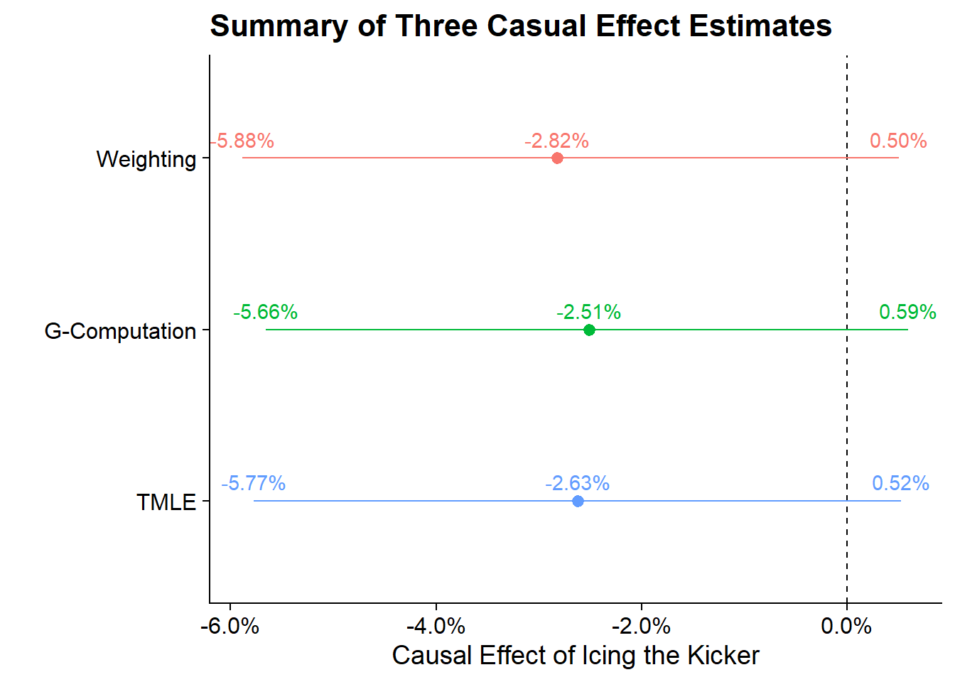
Altogether the three methodology align on the idea that icing the kicker is not a significant effect on the outcome of the Field Goal and even if it were (based on point estimate) it would be quite small.